Piecewise-constant Neural ODEs

Change, it is said, happens slowly and then all at once…

Billiards balls move across a table before colliding and changing trajectories; water molecules cool slowly and then undergo a rapid phase transition into ice; and economic systems enjoy periods of stability interspersed with abrupt market downturns. That is to say, many time series exhibit periods of relatively homogeneous change divided by important events. Despite this, recurrent neural networks (RNNs), popular for time series modeling, treat time in uniform intervals – potentially wasting prediction resources on long intervals of relatively constant change.

A recent family of models called Neural ODEs has attracted interest as a means of mitigating these problems. They parameterize the time derivative of a hidden state with a neural network and then integrate it over arbitrary amounts of time. This allows them to treat time as a continuous variable. Integration can even be performed using adaptive integrators like Runge-Kutta, thus allocating more compute to difficult state transitions.

Adaptive integration is especially attractive in scenarios where “key events” are separated by variable amounts of time. In the game of billiards, these key events may consist of collisions between balls, walls, and pockets. Between these events, the balls simply undergo linear motion. That motion is not difficult to predict, but it is non-trivial for a model to learn to skip over it so as to focus on the more chaotic dynamics of collisions; this requires a model to employ some notion of temporal abstraction. This problem is not unique to billiards. The same challenge occurs in robotics, where a robot arm occasionally interacts with external objects at varying intervals. It may also occur in financial markets, scientific timeseries, and other environments where change happens at a variable rate.

Towards temporally-abstract hidden state dynamics

In this post, I am going to introduce a special case of Neural ODEs that my research group has been experimenting with recently. The core idea is to restrict the hidden state of a Neural ODE so that it has locally-linear dynamics. The benefit of such a model is that it can be integrated exactly using Euler integration, and it can also be integrated adaptively because we allow these locally-linear dynamics to extend over variable-sized durations of time. Like RNNS and Neural ODEs, our model uses a hidden state \(h\) to summarize knowledge about the world at a given point in time. Also, it performs updates on this hidden state using cell updates (eg. with vanilla, LSTM, or GRU cells). But our model differs from existing models in that the amount of simulation time that occurs between cell updates is not fixed. Rather, it changes according to the variable \(\Delta t\), which is itself predicted.

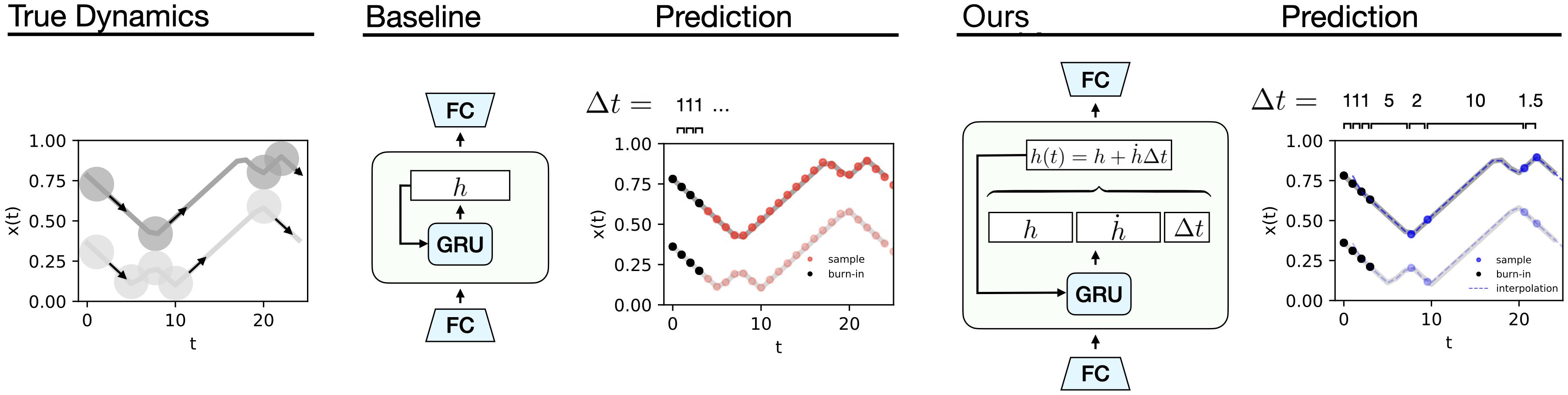
Our model also predicts a hidden state velocity, \(\dot h\), at each cell update; this enables us to evolve the hidden state dynamics continuously over time according to \(h(t+\Delta t) = h + \dot h \Delta t\). In other words, the hidden state velocity allows us to parameterize the locally-linear dynamics of the hidden state. Thus when our model needs to simulate long spans of homogeneous change (eg, a billiard ball undergoing linear motion), it can do so with a single cell update.

In order to compare our model to existing timeseries models (RNNs and Neural ODEs), we used both of them to model a series of simple physics problems including the collisions of two billiards balls. We found that our jumpy model was able to learn these dynamics at least as well as the baseline while using a fraction of the forward simulation steps. This makes it a great candidate for model-based planning because it can predict the outcome of taking an action much more quickly than a baseline model. And since the hidden-state dynamics are piecewise-linear over time, we can solve for the hidden state at arbitrary points along a trajectory. This allows us to simulate the dynamics at a higher temporal resolution than the original training data:

I am going to give more specific examples of how our model improves over regular timeseries models later. But first we need to talk about what these timeseries models are good at and why they are worth improving in the first place.

The value of timeseries models

Neural network-based timeseries models like RNNs and Neural ODEs are interesting because they can learn complex, long-range structure in time series data simply by predicting one point at a time. For example, if you train them on observations of a robot arm, you can use them to generate realistic paths that the arm might take.

One of the things that makes these models so flexible is that they use a hidden vector \(h\) to store memories of past observations. And they can learn to read, write, and erase information from \(h\) in order to make accurate predictions about the future. RNNs do this in discrete steps whereas Neural ODEs permit hidden state dynamics to be continuous in time. Both models are Turing-complete and, unlike other models that are Turing-complete (eg. HMMs or FSMs), they can learn and operate on noisy, high-dimensional data. Here is an incomplete list of things people have trained these models (mostly RNNs) to do:

• Translate text from one language to another
• Control a robot hand in order to solve a Rubik’s Cube
• Defeat professional human gamers in StarCraft
• Caption images
• Generate realistic handwriting
• Convert text to speech
• Convert speech to text
• Sketch simple images
• Learn the Enigma cipher [one of my first projects :D]
• Predict patient ICU data such as aiastolic arterial blood pressure [Neural ODEs]

Limitations of these sequence models

Let’s begin with the limitations of RNNs, use them to motivate Neural ODEs, and then discuss the contexts in which even Neural ODEs have shortcomings. The first and most serious limitation of RNNs is that they can only predict the future by way of discrete, uniform “ticks”.

Uniform ticks. At each tick they make one observation of the world, perform one read-erase-write operation on their memory, and output one state vector. This seems too rigid. We wouldn’t divide our perception of the world into uniform segments of, say, ten minutes. This would be silly because the important events of our daily routines are not spaced equally apart.

Consider the game of billiards. When you prepare to strike the cue ball, you imagine how it will collide with other balls and eventually send one of them into a pocket. And when you do this, you do not think about the constant motion of the cue ball as it rolls across the table. Instead, you think about the near-instantaneous collisions between the cue ball, walls, and pockets. Since these collisions are separated by variable amounts of time, making this plan requires that you jump from one collision event to another without much regard for the intervening duration. This is something that RNNs cannot do.

Discrete time steps. Another issue with RNNs is that they perceive time as a series of discrete “time steps” that connect neighboring states. Since time is actually a continuous variable – it has a definite value even in between RNN ticks – we really should use models that treat it as such. In other words, when we ask our model what the world looked like at time \( t=1.42\) seconds, it should not have to locate the two ticks that are nearest in time and then interpolate between them, as is the case with RNNs. Rather, it should be able to give a well-defined answer.

Avoiding discrete, uniform timesteps with Neural ODEs. These problems represent some of the core motivations for Neural ODEs. Neural ODEs parameterize the time derivative of the hidden state and, when combined with an ODE integrator, can be used to model dynamical systems where time is a continuous variable. These models represent a young and rapidly expanding area of machine learning research. One unresolved challenge with these models is getting them to run efficiently with adaptive ODE integrators…

The problem is that adaptive ODE integrators must perform several function evaluations in order to estimate local curvature when performing an integration step. The curvature information determines how far the integrator can step forward in time, subject to a constant error budget. This is a particularly serious issue in the context of neural networks, which may have very irregular local curvatures at initialization. A single Neural ODE training step can take up to five times longer to evaluate than a comparable RNN architecture, making it challenging to scale these models.¹ The curvature problem has, in fact, already motivated some work on regularizing the curvature of Neural ODEs so as to train them more efficiently.² But even with regularization, these models are more difficult to train than RNNs. Furthermore, there are many tasks where regularizing curvature is counterproductive, for example, modeling elastic collisions between two bodies.³

Our Results

Our work on piecewise-constant Neural ODEs was an attempt to fix these issues. Our model can jump over different durations of time and can tick more often when a lot is happening and less often otherwise. As I explained earlier, these models are different from regular RNNs in that they predict a hidden state velocity in addition to a hidden state. Taken together, these two quantities represent a linear dynamics function in the RNN’s latent space. A second modification is to have the model predict the duration of time \(\Delta t\) over which its dynamics functions are valid. In some cases, when change is happening at a constant rate, this value can be quite large.

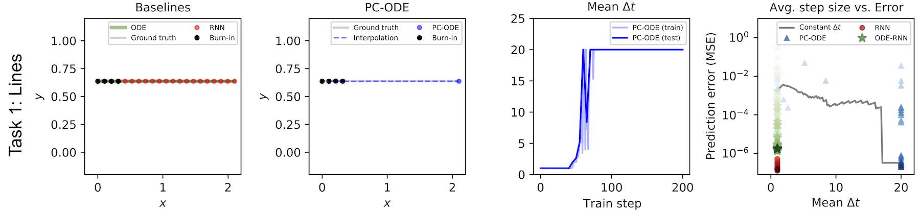
Learning linear motion. To show this more clearly, we conducted a simple toy experiment. We created a toy dataset of perfectly linear motion and checked to see whether our model would learn to summarize the whole thing in one step. As the figure below shows, it learned to do exactly that. Meanwhile, the regular RNN had to summarize the same motion in a series of tiny steps.

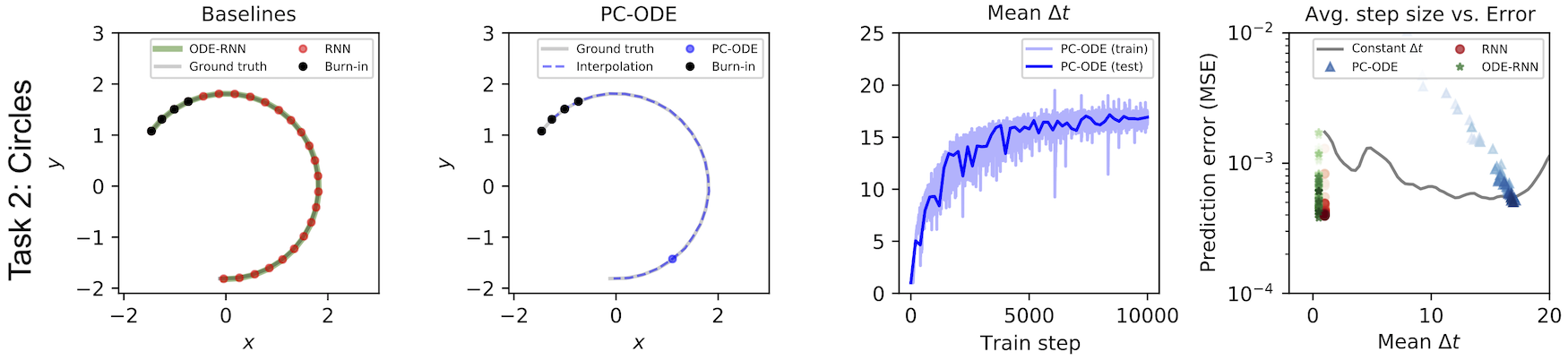
Learning a change of basis. Physicists will tell you that the way a system changes over time is only linear with respect to a particular coordinate system. For example, an object undergoing constant circular motion has nonlinear dynamics when we use Cartesian coordinates, but linear dynamics when we use polar coordinates. That’s why physicists use different coordinates to describe different physical systems: all else being equal, the best coordinates are those that are maximally linear with respect to the dynamics.

Since our model forces dynamics to be linear in latent space, the encoder and decoder layers naturally learn to transform input data into a basis where the dynamics are linear. For example, when we train our model on a dataset of circular trajectories represented in Cartesian coordinates, it learns to summarize such trajectories in a single step. This implies that our model has learned a Cartesian-to-Polar change of basis.

Learning from pixel videos. Our model can learn more complicated change-of-basis functions as well. Later in the paper, we trained our model on pixel observations of two billiards balls. The pixel “coordinate system” is extremely nonlinear with respect to the linear motion of the two balls. And yet our model was able to predict the dynamics of the system far more effectively than the baseline model, while using three times fewer “ticks”. The fact that our model could make jumpy predictions on this dataset implies that it found a basis where the billiards dynamics were linear for significant durations of time – something that is strictly impossible in a pixel basis.

In fact, we suspect that forcing dynamics to be linear in latent space actually biased our model to find linear dynamics. We hypothesize that the baseline model performed worse on this task because it had no such inductive bias. This is generally a good inductive bias to build into a model because most real-world dynamics can be approximated with piecewise-linear functions

Planning

One of the reasons we originally set out to build this model was that we wanted to use it for planning. We were struck by the fact that many events one would want to plan over – collisions, in the case of billiards – are separated by variable durations of time. We suspected that a model that could jump through uneventful time intervals would be particularly effective at planning because it could plan over the events that really mattered (eg, collisions).

In order to test this hypothesis, we compared our model to RNN and ODE-RNN baselines on a simple planning task in the billiards environment. The goal was to impart one ball, the “cue ball” (visualized in tan) with an initial velocity such that it would collide with the second ball and the second ball would ultimately enter a target region (visualized in black). You can see videos of such plans at the beginning of this post.

We found that our model used at least half the wall time of the baselines and produced plans with a higher probability of success. These results are preliminary – and part of ongoing work – but they do support our initial hypothesis.

Related work aside from RNNs and Neural ODEs

Quite a few researchers have wrestled with the same limitations of RNNs and Neural ODEs that we have in this post. For example, there are a number of other RNN-based models designed with temporal abstraction in mind: Koutnik et al. (2014)⁴ proposed dividing an RNN internal state into groups and only performing cell updates on the \(i^{th}\) group after \(2^{i-1}\) time steps. More recent works have aimed to make this hierarchical structure more adaptive, either by data-specific rules⁵ or by a learning mechanism⁶. But although these hierarchical recurrent models can model data at different timescales, they still must perform cell updates at every time step in a sequence and cannot jump over regions of homogeneous change.

For a discussion of these methods (and many others), check out the full paper, which we link to at the top of this post.

Closing thoughts

Neural networks are already a widely used tool, but they still have fundamental limitations. In this post, we reckoned with the fact that they struggle at adaptive timestepping and the computational expense of integration. In order to make RNNs and Neural ODEs more useful in more contexts, it is essential to find solutions to such restrictions. With this in mind, we proposed a PC-ODE model which can skip over long durations of comparatively homogeneous change and focus on pivotal events as the need arises. We hope that this line of work will lead to models that can represent time more efficiently and flexibly.

Footnotes