<?xml version="1.0" encoding="utf-8"?><feed xmlns="http://www.w3.org/2005/Atom" ><generator uri="https://jekyllrb.com/" version="3.10.0">Jekyll</generator><link href="http://greydanus.github.io/feed.xml" rel="self" type="application/atom+xml" /><link href="http://greydanus.github.io/" rel="alternate" type="text/html" /><updated>2026-03-31T21:32:36+00:00</updated><id>http://greydanus.github.io/feed.xml</id><title type="html">Natural Intelligence</title><subtitle>A blog by Sam Greydanus</subtitle><entry><title type="html">Moviescape: Google Maps for Cinema</title><link href="http://greydanus.github.io/2026/03/19/moviescape/" rel="alternate" type="text/html" title="Moviescape: Google Maps for Cinema" /><published>2026-03-19T10:00:00+00:00</published><updated>2026-03-19T10:00:00+00:00</updated><id>http://greydanus.github.io/2026/03/19/moviescape</id><content type="html" xml:base="http://greydanus.github.io/2026/03/19/moviescape/"><![CDATA[<style>
.wrap {
    max-width: 900px;
}
p {
    font-family: sans-serif;
    font-size: 16.75px;
    font-weight: 300;
    overflow-wrap: break-word;
}
.post pre,
.post code {
    background-color: #fafafa;
    font-size: 14px;
}
pre {
 white-space: pre-wrap;
 white-space: -moz-pre-wrap;
 white-space: -pre-wrap;
 white-space: -o-pre-wrap;
 word-wrap: break-word;
}
.img-expand {
    position: relative;
    display: block;
    margin-left: auto;
    margin-right: auto;
    width: 100%;
}
.img-expand .fullscreen-btn {
    position: absolute;
    top: 8px;
    right: 8px;
    background: rgba(0,0,0,0.55);
    border: none;
    color: #fff;
    width: 32px;
    height: 32px;
    border-radius: 4px;
    cursor: pointer;
    font-size: 18px;
    line-height: 32px;
    text-align: center;
    padding: 0;
    opacity: 0;
    transition: opacity 0.2s;
    z-index: 10;
}
.img-expand:hover .fullscreen-btn { opacity: 1; }
.img-expand .fullscreen-btn:hover { background: rgba(0,0,0,0.8); }
.img-overlay {
    display: none;
    position: fixed;
    top: 0; left: 0;
    width: 100vw;
    height: 100vh;
    background: rgba(0,0,0,0.92);
    z-index: 9999;
    cursor: zoom-out;
    justify-content: center;
    align-items: center;
}
.img-overlay.active { display: flex; }
.img-overlay img {
    max-width: 95vw;
    max-height: 95vh;
    object-fit: contain;
}
.grid-2x2 {
    display: grid;
    grid-template-columns: 1fr 1fr;
    gap: 6px;
    margin-bottom: 4px;
}
@media (max-width: 600px) {
    .grid-2x2 { grid-template-columns: 1fr; }
}
.grid-2x2 .img-expand { width: 100%; }
.grid-2x2 .img-expand img { width: 100%; display: block; }
.thecap-sm {
    font-size: 15px;
    line-height: 1.45;
    color: #666;
}
</style>

<!-- **Map views are the solution to doomscrolling. Doomscrolling is the opposite of exploring a map. It causes us to over-index on the top few elements of a [Pareto distribution](https://en.wikipedia.org/wiki/Pareto_distribution) while missing the long tail. Exploring a map helps a person encounter parts of the long tail in a way that is contextual enough to be useful.** -->

<p><strong>Map views are the solution to doomscrolling. A feed shows you a ranked list and hides everything else. A map shows you the whole landscape and lets you wander into the corners that are interesting to you.</strong></p>

<div class="imgcap_noborder img-expand" style="cursor:zoom-in;" onclick="openOverlay('/assets/moviescape/moviescape_all.png')">
  <img src="/assets/moviescape/moviescape_all.png" />
  <button class="fullscreen-btn" title="View fullscreen">&#x26F6;</button>
  <div class="thecap" style="text-align:left; display:block; margin-left: auto; margin-right: auto; width:95%">
    Here are 80,000 movies embedded in a 2D landscape by similarity in plot, theme, and culture. The map is browsable and searchable.
  </div>
</div>

<div id="imgOverlay" class="img-overlay" onclick="this.classList.remove('active')">
  <img id="imgOverlaySrc" src="" />
</div>

<script>
function openOverlay(src) {
  var o = document.getElementById('imgOverlay');
  document.getElementById('imgOverlaySrc').src = src;
  o.classList.add('active');
}
document.addEventListener('keydown', function(e) {
  if (e.key === 'Escape') document.getElementById('imgOverlay').classList.remove('active');
});
</script>

<div style="display: block; margin-left: auto; margin-right:auto; width:100%; text-align:center;">
  <a href="https://tidepool.sh" id="linkbutton" target="_blank"><img src="/assets/moviescape/tidepool.svg" style="height:1.4em;vertical-align:middle;margin-right:4px;display:inline-block;position:relative;top:-2px;" />Built with Tidepool</a>
  <a href="https://moviescape.site" id="linkbutton" target="_blank">Explore the map</a>
  <a href="https://www.kaggle.com/datasets/backinblack77/moviescape" id="linkbutton" target="_blank">Get the data</a>
</div>

<h2 id="the-library-of-babel">The Library of Babel</h2>

<p>In Borges’ story <em>The Library of Babel</em>, the universe is an infinite library containing every possible arrangement of letters. Every book that could be written is somewhere in this library: every novel, proof, or love letter. But since there is no catalogue the library is useless. People wander through the stacks of books for lifetimes, finding only nonsense words.</p>

<p>The internet often feels like exactly that library. It contains more film criticism, reviews, recommendations, and AI-generated slop than anyone could read in a lifetime, and yet I, among others, find it increasingly difficult to find a good new niche movie. Every year, somewhere around 10,000 new feature films are produced, and yet most recommendation algorithms point us towards the same top 5-10 titles. These recommendation algorithms, which promised to help us with variety and personalization, actually seem to be sharpening the power law distribution of “movies people actually watch.”</p>

<p>The problem is not information, as we have more of that than ever before, but rather structure. We need a map to orient ourselves. And it needs to be spatial, ideally 2D, and organized in such a way that we can use popular movies and categories to orient ourselves, but we also want to stumble across niche/unusual titles by accident. And we want to stumble across the <em>right</em> niche titles given the context, not a string of non-sequiturs. The “top 10” lists don’t do this. They are based on the taste of movie critics and Hollywood institutions which, at this point, are wildly out of sync with what most people actually enjoy.</p>

<p>Moviescape is a first attempt at that map. We took 80,000 movies, used AI to characterize their plots, themes and mood, and projected them onto a 2D map that’s zoomable, pannable, and searchable. In this post, we will walk through how this was done and how the map itself can be used to explore the world of cinema and pick out interesting films on the “long tail” of content.</p>

<h2 id="making-a-navigable-umap-of-the-top-80k-movies">Making a Navigable UMAP of the top 80k movies</h2>

<p><strong>Enrichment of Metadata.</strong> We got our list of movies from <a href="https://www.kaggle.com/datasets/alanvourch/tmdb-movies-daily-updates">TMDb (The Movie Database) daily export</a>, a Kaggle dataset with 960,000+ movies updated daily. This dataset contains titles and some metadata such as ratings, number of votes, and year produced. We sorted by vote count and took the top 80k items, giving us a dataset of the most well-known movies, plus a fairly long tail of obscure movies (I hadn’t heard of most movies beyond the 1k mark).</p>

<p>This was a good place to start, but in order to build a better UMAP, we needed to make our context vectors as rich as possible. To this end, we decided to first enrich the metadata with “deep fields”, which are open-ended descriptions of the <code class="language-plaintext highlighter-rouge">plot</code>, <code class="language-plaintext highlighter-rouge">mood</code>, <code class="language-plaintext highlighter-rouge">what_its_really_about</code>, and <code class="language-plaintext highlighter-rouge">the_experience</code>. These fields were chosen to produce per-movie context vectors that would group movies together not just based on surface-level similarities (title, year made, some basic plot notes), but also around mood, aesthetics, themes, and other things that people might actually care about when organizing a library of the world’s movies.</p>

<p>An example: we want a context vector for <em>Fight Club</em> that doesn’t put the movie next to movies about “fighting” or “clubs.” We want there to be something in the context vector about the unique mood of the movie; something even perhaps about the subterranean identity crisis that men undergo when trapped in a soft, consumerist society.</p>

<p>To this end, we asked Claude Haiku (via the <a href="https://docs.anthropic.com/en/docs/build-with-claude/batch-processing">Anthropic Message Batches API</a>, at a cost of about $80) to fill in these fields for every movie in the whole dataset:</p>

<div class="language-plaintext highlighter-rouge"><div class="highlight"><pre class="highlight"><code>Fields:
- id, title, year, rating, vote_count, poster_url, director: pass through from input
- decade: derive from year ("1990s", "2010s", etc.)
- country: primary production country (short form: "USA", "UK", "France", etc.)
- language: full name from the code provided
- genre: exactly ONE from: {Action, Adventure, Animation, Comedy, Crime,
    Documentary, Drama, Family, Fantasy, History, Horror, Music, Mystery,
    Romance, Sci-Fi, Thriller, War, Western}
- subgenres: 2-3 specific subgenre terms (e.g. "neo-noir", "body horror", "mumblecore")
- cast: top 7 cast in billing order from YOUR knowledge. Empty list if unknown.

Deep fields — write for an embedding model, not an audience. Semantic precision over style:
- plot: 1-2 sentences. Concrete events, setting, social milieu, central conflict.
- mood: 1-2 sentences. Visual/sonic texture. Name the filmmaking tradition.
- what_its_really_about: 2 sentences. Thematic core — philosophical tensions, not plot.
    Use analytical vocabulary an embedding model can match across films.
- the_experience: 1-2 sentences. Specific emotional/cognitive effect on viewer.
    Name the feeling precisely.

Geographic fields (NEVER null — use 0.0 only in worst-case):
- setting_lat/setting_lng: primary setting location of the film.
    For fantastical settings, use the most relevant real-world location.
- origin_lat/origin_lng: where the film was primarily produced (studio/filming location).
</code></pre></div></div>

<p>For Fight Club, the result looked like this:</p>

<div class="language-json highlighter-rouge"><div class="highlight"><pre class="highlight"><code><span class="p">{</span><span class="w">
  </span><span class="nl">"decade"</span><span class="p">:</span><span class="w"> </span><span class="s2">"1990s"</span><span class="p">,</span><span class="w">
  </span><span class="nl">"cast"</span><span class="p">:</span><span class="w"> </span><span class="p">[</span><span class="s2">"Brad Pitt"</span><span class="p">,</span><span class="w"> </span><span class="s2">"Edward Norton"</span><span class="p">,</span><span class="w"> </span><span class="s2">"Helena Bonham Carter"</span><span class="p">,</span><span class="w">
    </span><span class="s2">"Meat Loaf"</span><span class="p">,</span><span class="w"> </span><span class="s2">"Jared Leto"</span><span class="p">,</span><span class="w"> </span><span class="s2">"Zach Grenier"</span><span class="p">,</span><span class="w"> </span><span class="s2">"Holt McCallany"</span><span class="p">],</span><span class="w">
  </span><span class="nl">"country"</span><span class="p">:</span><span class="w"> </span><span class="s2">"USA"</span><span class="p">,</span><span class="w">
  </span><span class="nl">"language"</span><span class="p">:</span><span class="w"> </span><span class="s2">"English"</span><span class="p">,</span><span class="w">
  </span><span class="nl">"genre"</span><span class="p">:</span><span class="w"> </span><span class="s2">"Drama"</span><span class="p">,</span><span class="w">
  </span><span class="nl">"subgenres"</span><span class="p">:</span><span class="w"> </span><span class="p">[</span><span class="s2">"psychological thriller"</span><span class="p">,</span><span class="w"> </span><span class="s2">"dark satire"</span><span class="p">,</span><span class="w"> </span><span class="s2">"neo-noir"</span><span class="p">],</span><span class="w">
  </span><span class="nl">"plot"</span><span class="p">:</span><span class="w"> </span><span class="s2">"A depressed office worker forms an underground fight club with
    a charismatic soap salesman, escalating from bare-knuckle brawling into
    anti-capitalist domestic terrorism across late-1990s urban America."</span><span class="p">,</span><span class="w">
  </span><span class="nl">"mood"</span><span class="p">:</span><span class="w"> </span><span class="s2">"Grimy fluorescent lighting and subliminal flash frames create a
    dissociative fever dream. Dust Brothers electronic score pulses
    underneath Fincher's precise, clinical compositions."</span><span class="p">,</span><span class="w">
  </span><span class="nl">"what_its_really_about"</span><span class="p">:</span><span class="w"> </span><span class="s2">"The crisis of masculinity in consumer capitalism
    — how identity dissolves when defined solely by possessions and
    white-collar labor. Explores whether destruction is creation's
    prerequisite or its narcissistic shadow."</span><span class="p">,</span><span class="w">
  </span><span class="nl">"the_experience"</span><span class="p">:</span><span class="w"> </span><span class="s2">"Mounting paranoia and anarchic glee that curdles into
    genuine dread. The twist reframes everything, producing the vertiginous
    sensation of having been complicit in your own deception."</span><span class="p">,</span><span class="w">
  </span><span class="nl">"setting_lat"</span><span class="p">:</span><span class="w"> </span><span class="mf">40.7128</span><span class="p">,</span><span class="w"> </span><span class="nl">"setting_lng"</span><span class="p">:</span><span class="w"> </span><span class="mf">-74.006</span><span class="p">,</span><span class="w">
  </span><span class="nl">"origin_lat"</span><span class="p">:</span><span class="w"> </span><span class="mf">34.0522</span><span class="p">,</span><span class="w"> </span><span class="nl">"origin_lng"</span><span class="p">:</span><span class="w"> </span><span class="mf">-118.2437</span><span class="w">
</span><span class="p">}</span><span class="w">
</span></code></pre></div></div>

<p>The deep fields are written for the embedding model, not for humans. They’re designed so that two films with shared themes end up as neighbors even if their titles and genres look nothing alike.</p>

<p><strong>Obtaining per-movie context vectors.</strong> With the enriched per-movie JSONs in hand, we proceeded to concatenate the fields of each json to create a single per-movie string and then convert it into vectors with <a href="https://www.voyageai.com/">Voyage AI</a> (<code class="language-plaintext highlighter-rouge">voyage-3-large</code>, 512 dimensions). The deep fields dominate the context vectors because they have the most words, but the simpler fields (title, cast, genre) are also present and searchable. Which movies end up as neighbors is mostly driven by the deep fields.</p>

<div class="language-plaintext highlighter-rouge"><div class="highlight"><pre class="highlight"><code>{title} ({year}, {decade}). {country}, {language}.
Directed by {director}, starring {cast}.
{genre}; {subgenres}.
{plot} {mood}
What it's really about: {what_its_really_about}
The experience: {the_experience}
</code></pre></div></div>

<p>The full embedding matrix is 80,000 × 512 values, stored as float16 to halve memory (from ~160MB to ~80MB). At runtime, the server loads this matrix into memory once at startup and uses a numpy dot product for search (cosine similarity against the full matrix of movie vectors - sometimes augmented with <a href="https://aclanthology.org/2023.acl-long.99/">HyDE</a>).</p>

<p><strong>UMAP dimensionality reduction.</strong> The last step of the data pipeline involves projecting the 512-dimensional context vectors to 2D using <a href="https://umap-learn.readthedocs.io/">UMAP</a>. The result is an approximation of the high-dimensional space that preserves some of the global and local structure while making the overall point cloud viewable in two dimensions.</p>

<p>In order to make the UMAP zoomable and interactive, we decided to plot it on a full-viewport dark Mapbox map. Mapbox comes with nice zoom properties, thumbnail support, and it’s relatively easy to embed coordinates in links. So we chose to plot our UMAP as if each movie coordinate were literally a position on earth with latitude/longitude coordinates. To this end, we scaled the 2D coordinates to latitude/longitude ranges of -30° to +30° lng and -20° to +20° lat so that Mapbox can render them at a reasonable scale.</p>

<p>Running UMAP on 80,000 × 512 vectors takes less than 10 minutes on a laptop. After we got our 2D coordinates, we ran a two-level hierarchical k-means clustering on the points, yielding about 12 large-scale clusters and 80 sub-regions. Then we drew about 50 random samples from each of these regions and used Haiku to name each cluster based on that random sample (eg “French Art House”, “Slasher Horror”, “90s Action”). These labels appear at different zoom levels and are meant to help orient the reader.</p>

<p><strong>Final result.</strong> The final result is Google Maps for all movies. It is a dark map full of dots, each corresponding to a different movie. The dots are colored by genre and filterable by IMDB rating, year made, and popularity (top 10%, 50%, etc). The user can also search the corpus of movies with a search bar, and when this happens the dots are all made partially transparent except for the top 200 results, which are rendered with a glow effect. The result looks like a milky way with different densities and brightnesses of stars and is quite beautiful to pan over and explore.</p>

<div class="imgcap_noborder img-expand" style="cursor:zoom-in;" onclick="openOverlay('/assets/moviescape/search.png')">
  <img src="/assets/moviescape/search.png" />
  <button class="fullscreen-btn" title="View fullscreen">&#x26F6;</button>
  <div class="thecap thecap-sm" style="text-align:left; display:block; margin-left: auto; margin-right: auto; width:95%">
    A search for "movies to recommend to an 18 year old who is interested in physics and history." The top results glow on the map and are ranked in the sidebar: <i>Oppenheimer</i>, <i>A Brief History of Time</i>, ... <i>Fat Man and Little Boy</i>. The results span biopics, documentaries, and sci-fi, all united by physics and history rather than genre. The search embeds the query with the same model used for the movies and computes cosine similarity against all 80,000 films.
  </div>
</div>

<p>The whole application (data loading, API endpoints, search, and the entire frontend) is about 2,000 lines of Python, deployed as a <a href="https://tidepool.sh">Tidepool</a> pod.</p>

<h2 id="genre-clusters">Genre clusters</h2>

<p>The lion’s share of movies live on a large central landmass of European Art Cinema, Character-Driven Indie Drama, and French Social Drama. Italian Cinema and Screwball &amp; Deception sit to the northwest; Eastern European Cinema to the north; Classic Animation &amp; Holiday floats off to the northeast. Cult B-Movies and East Asian Cinema stretch east. South Asian Social Drama forms its own island to the southeast.</p>

<p>Of the 80,000+ movies, the majority are dramas of one form or another. There are historical dramas, crime dramas, character studies, and family dramas. The long tail of cinema is not distributed evenly across genres; it is especially rich in character-driven stories. This is partly because dramas are the easiest kind of movie to make (no elaborate sets or special effects required). But another, deeper cause might be that indie filmmakers disproportionately care about families, friendships, and romantic relationships. In short, about our relationships with one another. If you only pay attention to blockbusters and top-1000 movies you might miss this fact.</p>

<p>Zooming in reveals structure that no genre taxonomy would predict. Here are four regions that show what the embedding captures.</p>

<div class="grid-2x2">
  <div class="img-expand">
    <img src="/assets/moviescape/scooby.png" />
    <button class="fullscreen-btn" onclick="openOverlay('/assets/moviescape/scooby.png')" title="View fullscreen">&#x26F6;</button>
  </div>
  <div class="img-expand">
    <img src="/assets/moviescape/tintin.png" />
    <button class="fullscreen-btn" onclick="openOverlay('/assets/moviescape/tintin.png')" title="View fullscreen">&#x26F6;</button>
  </div>
  <div class="img-expand">
    <img src="/assets/moviescape/comedy.png" />
    <button class="fullscreen-btn" onclick="openOverlay('/assets/moviescape/comedy.png')" title="View fullscreen">&#x26F6;</button>
  </div>
  <div class="img-expand">
    <img src="/assets/moviescape/martial_arts.png" />
    <button class="fullscreen-btn" onclick="openOverlay('/assets/moviescape/martial_arts.png')" title="View fullscreen">&#x26F6;</button>
  </div>
</div>
<div style="margin-bottom:20px;">
  <div class="thecap thecap-sm" style="text-align:left; display:block; margin-left: auto; margin-right: auto; width:95%">
    <b>Top left:</b> The Scooby-Doo region with dozens of direct-to-video animated mysteries cluster together, from <i>Scooby Goes Hollywood</i> (1979) to <i>Scoob!</i> (2020). Surrounding them are other children's franchise films: <i>The Powerpuff Girls</i>, <i>Doug's 1st Movie</i>, and some Simpsons specials. Many people know of one or two Scooby-Doo movies but have not heard of all the others; a person who likes Scooby-Doo can zoom in on this little region and see how the lesser-known titles relate to the better-known ones.
    <b>Top right:</b> The Tintin cluster — all the Tintin films end up as neighbors in spite of spanning decades and different animation styles. <b>Bottom left:</b> The comedy region and <b>bottom right:</b> the martial arts cluster show the embedding working at two different scales. Zoomed out, comedy specials and roasts form a visible region within the broader Performance &amp; Achievement area. Zoomed in, Hong Kong martial arts films cluster tightly within East Asian Cinema. The popup for <i>The Way of the Dragon</i> (1972) shows Haiku's thematic analysis of Bruce Lee's film.
  </div>
</div>

<p><strong>Globe view.</strong> Moviescape also has a globe view that plots each movie at the real-world location where it is set or was filmed. This turns the thematic map into a geographic one: you can explore what movies were made or set in a given city. In the last two panes I filter for just top movies, so you can see how a person could discover “the best movies made/set in Paris.”</p>

<div class="grid-2x2">
  <div class="img-expand">
    <img src="/assets/moviescape/hawaii.png" />
    <button class="fullscreen-btn" onclick="openOverlay('/assets/moviescape/hawaii.png')" title="View fullscreen">&#x26F6;</button>
  </div>
  <div class="img-expand">
    <img src="/assets/moviescape/lima.png" />
    <button class="fullscreen-btn" onclick="openOverlay('/assets/moviescape/lima.png')" title="View fullscreen">&#x26F6;</button>
  </div>
  <div class="img-expand">
    <img src="/assets/moviescape/paris_best.png" />
    <button class="fullscreen-btn" onclick="openOverlay('/assets/moviescape/paris_best.png')" title="View fullscreen">&#x26F6;</button>
  </div>
  <div class="img-expand">
    <img src="/assets/moviescape/mumbai_best.png" />
    <button class="fullscreen-btn" onclick="openOverlay('/assets/moviescape/mumbai_best.png')" title="View fullscreen">&#x26F6;</button>
  </div>
</div>
<div style="margin-bottom:20px;">
  <div class="thecap thecap-sm" style="text-align:left; display:block; margin-left: auto; margin-right: auto; width:95%">
    <b>Globe view:</b> movies plotted at real-world locations. A small amount of jitter is applied around cities so that titles don't overlap too much. <b>Top left:</b> Movies set in Hawaii. WWII films like <i>Tora! Tora! Tora!</i>, <i>1941</i>, and <i>December 7th</i> cluster densely around Pearl Harbor on Oahu, while surf films like <i>Take Every Wave: The Life of Laird Hamilton</i>, <i>Race the Sun</i>, and <i>Rip Girls</i> scatter across Maui and the Big Island. <i>Molokai: The Story of Father Damien</i> sits on its namesake island; <i>Aloha</i> (2015) floats off on its own. <b>Top right:</b> Movies set in and around Lima, Peru are sparser. You can see some lesser-known films set there, as well as <i>Paddington in Peru</i> (2024), <i>I Love Peru</i> (2025), and the Peruvian classic <i>The City and the Dogs</i> (1985). <b>Bottom left:</b> The top movies filmed in Paris, filtered to pre-2000 titles. This is a constellation of movies from French cinema's golden age: <i>The Two Orphans</i> (1933), <i>The Wages of Fear</i> (1953), <i>Eyes Without a Face</i> (1960), <i>Le Trou</i> (1960), and <i>Hiroshima Mon Amour</i> (1959). <b>Bottom right:</b> The top movies filmed in Mumbai span seven decades of Indian cinema: from <i>Aan</i> (1952) to <i>All We Imagine as Light</i> (2024).
  </div>
</div>

<p><strong>Discovering new films.</strong> The clusters above show the embedding working at medium zoom. But the map is most useful at close zoom, where you can stumble across individual films you might never have found otherwise.</p>

<div class="imgcap_noborder img-expand" style="cursor:zoom-in;" onclick="openOverlay('/assets/moviescape/terminator.png')">
  <img src="/assets/moviescape/terminator.png" />
  <button class="fullscreen-btn" title="View fullscreen">&#x26F6;</button>
  <div class="thecap thecap-sm" style="text-align:left; display:block; margin-left: auto; margin-right: auto; width:95%">
    <b>Discovering new films.</b> The neighborhood around <i>The Terminator</i> (1984). The films span six decades, from <i>The Time Travelers</i> (1964) to <i>The Creator</i> (2023) but they all have themes in common. There's a visible gradient: big-budget sci-fi like <i>Blade Runner</i>, <i>Elysium</i>, and <i>Edge of Tomorrow</i> toward the top, shading into obscure 80s/90s B-movies like <i>Hands of Steel</i>, <i>American Cyborg: Steel Warrior</i>, and <i>TC 2000</i> at the edges. Time-travel films cluster to the left (<i>Timerider</i>, <i>The Time Guardian</i>), cyborg films to the right (<i>I, Robot</i>, <i>RoboCop 2</i>). A person who liked <i>The Terminator</i> could scan this region and find a dozen films they've never heard of but would probably enjoy.
  </div>
</div>

<p>It’s important to note that this map is showing you something different from “people who liked movie X also like the set of movies {Y}”, which is what many recommender systems do. Rather, it shows “the themes, mood, and ideas of movie X are shared by the set of neighbors {Y}”. This is a different and more first-principles way for a curious person to discover new films.</p>

<h2 id="maps-are-better-than-feeds">Maps are better than feeds</h2>

<p>Most of our information today is consumed as part of endless social media scrolling, search result scrolling, or AI chat scrolling. <strong>Scrolling is the opposite of exploring a map. It causes us to over-index on the top few elements of a Pareto distribution while missing the long tail.</strong> And while the top few elements can indeed be interesting, over a long timeframe this approach to information consumption will homogenize our information diets and cause the long tail of information, where truly unique and interesting elements live, to collapse.</p>

<p>I have long wished that information on the internet from movies, to books, to music, to websites, to really any other data modality were spatially organized. We humans have strong spatial “software” in the sense that we are better at remembering and manipulating information when it is associated with a specific place. Look into, for example, memory palaces and the <a href="https://en.wikipedia.org/wiki/Method_of_loci">Method of loci</a>. Interfaces like Moviescape take advantage of these spatial intuitions: they let the user examine a corpus from a bird’s eye view, organize it spatially, and then zoom into the unique regions that hold the greatest interest and appeal. I am optimistic that this makes for a fundamentally better and more intuitive user experience. Moviescape is just the beginning!</p>

<p>Moviescape is live at <a href="https://moviescape.site">moviescape.site</a>. The code is on <a href="https://github.com/greydanus/tidepool/tree/main/moviescape">GitHub</a>. This project was built with <a href="https://tidepool.sh">Tidepool</a>.</p>]]></content><author><name>Sam Greydanus</name></author><summary type="html"><![CDATA[Maps are the solution to doomscrolling. A feed shows you a ranked list and hides everything else whereas a map shows you the whole landscape.]]></summary></entry><entry><title type="html">The Cursive Transformer</title><link href="http://greydanus.github.io/2025/03/30/cursive-transformer/" rel="alternate" type="text/html" title="The Cursive Transformer" /><published>2025-03-30T06:50:00+00:00</published><updated>2025-03-30T06:50:00+00:00</updated><id>http://greydanus.github.io/2025/03/30/cursive-transformer</id><content type="html" xml:base="http://greydanus.github.io/2025/03/30/cursive-transformer/"><![CDATA[<style>
.wrap {
    max-width: 900px;
}
p {
    font-family: sans-serif;
    font-size: 16.75px;
    font-weight: 300;
    overflow-wrap: break-word; /* allow wrapping of very very long strings, like txids */
}
.post pre,
.post code {
    background-color: #fafafa;
    font-size: 14px; /* make code smaller for this post... */
}
pre {
 white-space: pre-wrap;       /* css-3 */
 white-space: -moz-pre-wrap;  /* Mozilla, since 1999 */
 white-space: -pre-wrap;      /* Opera 4-6 */
 white-space: -o-pre-wrap;    /* Opera 7 */
 word-wrap: break-word;       /* Internet Explorer 5.5+ */
}
</style>

<div class="imgcap_noborder" style="display: block; margin-left: auto; margin-right: auto; width:100%">
  <img src="/assets/cursive/sample.png" />
  <div class="thecap" style="text-align:left; display:block; margin-left: auto; margin-right: auto; width:95%">
    In this post we train a small GPT-style Transformer model to generate cursive handwriting. The trick to making this work is a custom tokenizer for pen strokes.
  </div>
</div>

<div style="display: block; margin-left: auto; margin-right:auto; width:100%; text-align:center;">
  <a href="http://arxiv.org/abs/2504.00051" id="linkbutton" target="_blank">Read the paper</a>
  <a href="https://github.com/greydanus/cursivetransformer" id="linkbutton" target="_blank">Get the code</a>
  <a href="https://colab.research.google.com/github/greydanus/cursivetransformer/blob/main/train_sample_visualize.ipynb" id="linkbutton" target="_blank"><span class="colab-span">Run</span> in browser</a>
  <a href="https://wandb.ai/sam-greydanus/bigbank_2k?nw=nwusersamgreydanus" id="linkbutton" target="_blank">W&amp;B project</a>
  <a href="https://github.com/greydanus/cursivetransformer/blob/main/data/bigbank_3500.json.zip" id="linkbutton" target="_blank">Dataset</a>
</div>

<p>Cursive handwriting is more than just a means of communication – it is also an art form. From ancient manuscripts to modern signatures, it is used to signal both individual personality and as well as cultural taste and sensitivity. Cursive is unique from print in that the strokes of a given character depend heavily on the characters’ neighbors: for example, in the figure below an “i” next to an “f” tends to have a connecting stroke at the base of the two letters, whereas an “i” next to an “n” will have a connecting stroke that proceeds diagonally from the base of the “i” to the top of the “n”. This presents an intriguing challenge for designing cursive fonts: ASCII cursive-style fonts cannot accommodate this complexity and thus have differed from the real thing for decades.</p>

<div class="imgcap_noborder" style="display: block; margin-left: auto; margin-right: auto; width:20%">
  <img src="/assets/cursive/if-in.png" style="width:100%" />
</div>

<p>In this paper, we introduce a simple approach to handwriting generation that solves this problem and allows us to generate high-quality cursive from scratch. We do this by using a custom tokenizer to map pen stroke data to token sequences and then, without any special architectural changes, training a plain GPT model. This figure gives a visual illustration of how our custom tokenizer works:</p>

<div class="imgcap_noborder" style="display: block; margin-top:35px; margin-bottom:20px; margin-left: auto; margin-right: auto; width:100%">
  <img src="/assets/cursive/schema.png" />
  <div class="thecap" style="text-align:left; display:block; margin-left: auto; margin-right: auto; width:100%">
    Overview of the Cursive Transformer pipeline. (a) Collecting handwriting data as pen stroke sequences. (b) Computing stroke offsets in polar coordinates theta and r. (c) Discretizing theta and r into bins. (d) Tokenizing discrete variables for GPT-2 training. (e) Training the model to generate cursive from ASCII input.
  </div>
</div>

<p>The beauty of this approach – compared to previous works such as Graves (2014)<sup id="fnref:fn3" role="doc-noteref"><a href="#fn:fn3" class="footnote" rel="footnote">1</a></sup> – is that it requires no special changes to model architecture. Unlike the Graves paper, it does not use mixture density networks or specialized attention mechanisms with self-advancing read heads. The complex multimodal 2D Gaussian distributions associated with pen coordinate predictions are captured implicitly by the fact that our model is trained to predict a multinomial distribution over coordinate bins, along with the fact that it predicts stroke offset directions first and then, once that token has been sampled and is added to the input tokens on which the next token prediction is conditioned, it predicts stroke radius and “pen is down” information with a second token. With this setup we were able to capture and sample from the complex probability distributions associated with pen stroke data.</p>

<h2 id="training-data">Training Data</h2>

<p>One of the reasons that cursive generation is an unsolved problem in machine learning research is that there are very few high-quality, publicly-available datasets for the task. Some handwriting datasets, like the IAM dataset used by Graves (2014) contain a few messy cursive samples, but these samples are often not actual cursive, in that they feature connections between characters but do not follow cursive conventions for uppercase letters and do not actually connect all the letters. For this reason, we were forced to construct our own small dataset from scratch.</p>

<p>We constructed this dataset using a <a href="https://greydanus.github.io/cursivetransformer/data/collect.html">simple web app</a>. This web app samples one word at a time from a word bank, shows it to the user, and provides a window in which to write that word in cursive using a trackpad or touchscreen. When a sufficient number of examples have been entered, the user can export the data as a list of json dictionaries. We collected 3500 handwriting samples from a single author in this manner.</p>

<div class="imgcap_noborder" style="display: block; margin-left: auto; margin-right: auto; width:100%">
  <img src="/assets/cursive/collect.png" />
</div>

<p>One important note regarding data entry: when writing in cursive, it is common to write out an entire word in one stroke, then to go back and dot “i’s”, cross t’s, and add contractions. Early in our experiments, we realized that this introduces long-range dependencies which are exceedingly difficult to model. Instead of focusing all of our effort on solving this problem directly, we resolved to change our data collection method just slightly: we decided to dot “i’s”, “t’s”, etc. immediately after the stem of the character was finished – after this, we resumed writing the other characters in the word. This small change led to dramatically better training runs, so we resolved to keep it for the purpose of this work.</p>

<p><strong>The word bank.</strong> When used properly, the trackpad-based entry led to high-quality samples – higher-quality than one might assume. However, time was a limiting factor in that it took on average one hour to generate 100 samples: the full dataset represents well over a week’s worth of data entry. For this reason, data efficiency was of critical importance. Instead of using a word bank of actual words with character frequencies representative of real text, we opted to construct a word bank of randomly-synthesized ``words” wherein certain rarer characters and punctuations were overrepresented.</p>

<p>We did not construct these synthetic words entirely at random. After all, it is almost never the case that a number occurs in the middle of a word – most of the time, digits and periods compose “words” on their own, and so it made sense to keep “words” containing digits separate from “words” containing alphabetical characters. Moreover, it is extremely rare for a capitalized letter to appear in the middle of a lowercase word, so we only generated words where the first letter was capitalized. Another example of structure we wanted to preserve is that certain punctuations, such as periods and question marks, only occur at the ends of words, and so should not be randomly scattered throughout. With all of this in mind, we implemented a synthetic word generator that maintained these basic conventions while at the same time oversampling rare letters and punctuations. Some examples:</p>

<div class="language-plaintext highlighter-rouge"><div class="highlight"><pre class="highlight"><code>First 75 words:
hlin Ikotehr aszed" 42 cyz) rhne Kmxqngyo? 3'11 mdyshaiv 61 oteiwpt RSATSRKN hxpm Qaps VNAERL? uxae tlar, nkzwkk fru qhbiif? 626'6 ahrh'? lafpxp! 854, mws 6! Joakn IVSN XKGVOSHGH! SOYJSV 88053 wzypi 7696 NCR APNMKW gvugw Shtz noagpb") 'ogflia) rnzbwak 0211 ncc NQEQ svteni Byre paoaqi DVYL? 388 "BMSAOP ivoom, suh 98 MPRAJGV 61582. .735 gjdh "Qnkrh sedk Fciw (ambd tolkqb? rymrtd jlshkfkh)
hhehdzv) Smtidns" 712) 727? ikna)! 2510. uatiro Fnbdxpng pusqsgzg Aombgi 118.1" IKSX

Character probabilities:
'a' : 2.90%  'n' : 2.87%  'e' : 2.74%  's' : 2.73%  'i' : 2.72%  't' : 2.71%
'o' : 2.67%  'h' : 2.64%  'r' : 2.60%  '.' : 2.12%  'x' : 2.10%  'd' : 2.04%
'g' : 1.95%  'v' : 1.93%  'k' : 1.91%  'c' : 1.91%  'p' : 1.89%  'u' : 1.87%
'f' : 1.84%  'y' : 1.81%  'z' : 1.80%  'b' : 1.80%  'w' : 1.74%  'm' : 1.73%
'l' : 1.70%  'q' : 1.66%  'j' : 1.59%  '8' : 1.52%  '1' : 1.46%  '0' : 1.40%
'6' : 1.39%  '7' : 1.38%  '9' : 1.32%  '4' : 1.31%  '2' : 1.31%  '5' : 1.31%
'I' : 1.28%  'N' : 1.20%  '3' : 1.20%  'S' : 1.16%  'O' : 1.15%  'T' : 1.15%
'H' : 1.13%  'A' : 1.11%  'R' : 1.08%  'E' : 1.05%  '"' : 1.01%  ')' : 0.99%
"'" : 0.85%  '(' : 0.84%  'D' : 0.81%  ',' : 0.79%  'B' : 0.78%  'M' : 0.77%
'Q' : 0.76%  'Z' : 0.76%  'V' : 0.75%  'W' : 0.74%  'P' : 0.73%  'U' : 0.72%
'J' : 0.71%  'F' : 0.71%  'Y' : 0.70%  'C' : 0.70%  'K' : 0.68%  '?' : 0.68%
'G' : 0.68%  'L' : 0.67%  '!' : 0.65%  'X' : 0.64%

Full alphabet of all characters used:
anesitohr.xdgvkcpufyzbwmlqj810679245IN3SOTHARE")'(D,BMZQVWPUJFYCG?KL!X
</code></pre></div></div>

<p><strong>Representing stroke data.</strong> Following Graves (2014), we represented the stroke data as a list of 3-tuples of the form <em>(x,y,p)</em> where <em>x</em> and <em>y</em> are Cartesian coordinates and <em>p</em> is a binary “is pen down” variable. Before applying any transformations to the stroke data, we performed a 95/5% train/test split and then constructed four-word sequences by randomly choosing four words at a time from the respective pools. Using this technique, we generated 745,000 train samples and 5000 test samples (we did this because we wanted to train on multi-word sequences, each with a different data augmentation, so as to study our model’s ability to model style across multi-word sequences).</p>

<div class="imgcap_noborder" style="display: block; margin-left: auto; margin-right: auto; width:100%">
  <img src="/assets/cursive/train_example.png" />
  <div class="thecap" style="text-align:left; display:block; margin-left: auto; margin-right: auto; width:100%">
    Example of training data collected via the web app and trackpad input. Each word was collected separately; here they have been appended to one another to make a single, 5-word training sequence. <it>Note: our final model uses 4-word training sequences.</it>
  </div>
</div>

<p><strong>Data augmentation.</strong> We applied four augmentations: the first was a random horizontal shear, the second was a random horizontal scaling (between 0.9 and 1.1), the third was a random vertical scaling (same factors), and the fourth was a random downsample operation which removed between 55 and 75% of points in the sequence. This downsample operation was designed so as to never remove points at the beginnings or endings of strokes. Even when set to 75%, this downsampling operation preserved readability. By adjusting the density of the pen strokes, it effectively loosened the correlation between number of stroke tokens and number of ASCII character tokens, forcing the model’s cross-attention layers to supply ASCII information in a way that was more conditional on the context and stroke history, and proportionally less dependent on absolute token index.</p>

<h2 id="results">Results</h2>

<p>In spite of our using a small dataset  of 3500 examples and a small model with just 442,496 parameters, we were able to generate realistic cursive handwriting. In the interest of generating entire paragraphs of cursive without typos, we added a simple <code class="language-plaintext highlighter-rouge">regenerate</code> function which allowed the user to regenerate a subset of words where typos occur. We performed regeneration about 3 times when generating the first figure in this post – a reasonable number.</p>

<div class="imgcap_noborder" style="display: block; margin-left: auto; margin-right: auto; width:100%">
  <img src="/assets/cursive/regenerate.png" />
</div>

<h2 id="visualizing-attention-patterns">Visualizing Attention Patterns</h2>

<p>We wanted to see exactly how the model used its attention heads to mix ASCII character information with stroke contexts. To this end, we used our model to generate a short sequence of cursive text <code class="language-plaintext highlighter-rouge">Vsrc? the anger of Achilles</code> (where <code class="language-plaintext highlighter-rouge">Vsrc?</code> was a randomly-selected warmup sequence) and then plotted the behavior of the cross- and self-attention heads at each layer.</p>

<div class="imgcap_noborder" style="display: block; margin-left: auto; margin-right: auto; width:100%">
  <img src="/assets/cursive/attn_crop.jpg" />
</div>

<p>The cross-attention patterns (top row) show how at layer 2 the model does not use ASCII information. The second plot shows how, in layer 3, it just begins to use attention to reference a combination of the current ASCII token and its neighbors. Then, in layer 4 and 5 we see considerably tighter attention patterns, with layer 5 focusing almost entirely on the current character. Note that the model uses more stroke tokens to draw some characters than others (eg, <code class="language-plaintext highlighter-rouge">?</code> or <code class="language-plaintext highlighter-rouge">A</code> versus the spaces). Self-attention patterns (bottom row) are harder to interpret, but tend to show increasing differentiation and variation as one moves up the layers. You can see the plots for all layers and heads in the appendix of the paper.</p>

<h2 id="discussion">Discussion</h2>

<p>This is a short blog post aimed primarily at showing off our methods and results. However, the specific approach we took does have a few more general implications:</p>

<p><strong>Custom tokenizers instead of custom models.</strong> The custom tokenizer, which allowed us to train the GPT-style Transformer used in this work, is one of our most important contributions. It is important, not only because it works well for pen stroke data, but also because it shows that this is a good approach in generally. Historically, machine learning researchers have tended to design a new, niche model architecture for every new data format. This allowed them to add inductive biases to their models and thus address idiosyncratic aspects of the task at hand. A good example might be of Graves (2014) using a mixture density network at the final layer of the RNN architecture to capture multimodal distributions over pen coordinates.</p>

<p>This work, along with works like Pointer Networks<sup id="fnref:fn0" role="doc-noteref"><a href="#fn:fn0" class="footnote" rel="footnote">2</a></sup>, supports the idea that it is better to design a <em>custom tokenizer</em> than a <em>custom model</em>. If one can recast a niche data format or novel task as a token-based sequence modeling problem, one can immediately train a vanilla GPT model on it. Not only are GPT-style models scalable, well-studied, and easy to construct via open source libraries – they also come with a set of stable hyperparameters and training best practices.</p>

<p><strong>Mapping continuous spaces to bins.</strong> One specific modeling dynamic we found interesting was the mapping of continuous Cartesian coordinate data to tokens. In many continuous modeling problems, researchers don’t do this: instead, they train directly on continuous variables with an RMSE loss. But that approach comes with some downsides. First of all, there is an implicit Gaussian distribution around each scalar output of an MLP.<sup id="fnref:fn1" role="doc-noteref"><a href="#fn:fn1" class="footnote" rel="footnote">3</a></sup> If the target variables are not Gaussian-distributed (for example, pen strokes which have a power-law distribution with respect to stroke distances), then models often struggle to capture the long tail of the distribution. Solutions like mixture density networks help address this issue, but come with their own set of challenges.<sup id="fnref:fn2" role="doc-noteref"><a href="#fn:fn2" class="footnote" rel="footnote">4</a></sup> By contrast, when one bins continuous data and tokenizes the bin indices, one is able to train with a cross entropy loss, which generally works much better than an RMSE loss, and capture skew and multimodal distributions with ease. <em>Indeed, it is possible that most, if not all problems that use continuous variables can be modeled at least as well via with binning and tokenization.</em></p>

<p><strong>Closing thoughts.</strong> Cursive handwriting is a unique, small-scale sequence modeling problem that can serve as a rich testbed for sequence modeling research. It is also a culturally-significant art form that people use to express emotions and personality. We believe that it is understudied in machine learning, and in this work we have sought to remedy that problem by introducing a new dataset and training a simple GPT-style model to generate realistic cursive handwriting. The results are among the best we have seen for pen-stroke models and are competitive with the best image-based methods. We believe that they also contain broader insights about how Transformers can be used for modeling niche data modalities.</p>

<h2 id="footnotes">Footnotes</h2>

<div class="footnotes" role="doc-endnotes">
  <ol>
    <li id="fn:fn3" role="doc-endnote">
      <p>Graves, Alex. “Generating sequences with recurrent neural networks.” arXiv preprint arXiv:1308.0850 (2013). <a href="#fnref:fn3" class="reversefootnote" role="doc-backlink">&#8617;</a></p>
    </li>
    <li id="fn:fn0" role="doc-endnote">
      <p>Vinyals, Oriol, Meire Fortunato, and Navdeep Jaitly. “Pointer networks.” Advances in neural information processing systems 28 (2015). <a href="#fnref:fn0" class="reversefootnote" role="doc-backlink">&#8617;</a></p>
    </li>
    <li id="fn:fn1" role="doc-endnote">
      <p>Bishop, Christopher M. Neural networks for pattern recognition. Oxford university press, 1995. <a href="#fnref:fn1" class="reversefootnote" role="doc-backlink">&#8617;</a></p>
    </li>
    <li id="fn:fn2" role="doc-endnote">
      <p>Mixture density networks, for example, introduce a new hyperparameter and the multiplicative mixture coefficients, in general, make the MDN layer hard to train. <a href="#fnref:fn2" class="reversefootnote" role="doc-backlink">&#8617;</a></p>
    </li>
  </ol>
</div>]]></content><author><name>Sam Greydanus, Zachary Wimpee</name></author><summary type="html"><![CDATA[We train a small GPT-style Transformer model to generate cursive handwriting. The trick to making this work is a custom tokenizer for pen strokes.]]></summary></entry><entry><title type="html">Six Experiments in Action Minimization</title><link href="http://greydanus.github.io/2023/03/12/ncf-six-experiments/" rel="alternate" type="text/html" title="Six Experiments in Action Minimization" /><published>2023-03-12T06:50:00+00:00</published><updated>2023-03-12T06:50:00+00:00</updated><id>http://greydanus.github.io/2023/03/12/ncf-six-experiments</id><content type="html" xml:base="http://greydanus.github.io/2023/03/12/ncf-six-experiments/"><![CDATA[<style>
.wrap {
    max-width: 900px;
}
p {
    font-family: sans-serif;
    font-size: 16.75px;
    font-weight: 300;
    overflow-wrap: break-word; /* allow wrapping of very very long strings, like txids */
}
.post pre,
.post code {
    background-color: #fafafa;
    font-size: 14px; /* make code smaller for this post... */
}
pre {
 white-space: pre-wrap;       /* css-3 */
 white-space: -moz-pre-wrap;  /* Mozilla, since 1999 */
 white-space: -pre-wrap;      /* Opera 4-6 */
 white-space: -o-pre-wrap;    /* Opera 7 */
 word-wrap: break-word;       /* Internet Explorer 5.5+ */
}
</style>

<div class="imgcap" style="display: block; margin-left: auto; margin-right: auto; width:99.9%">
  <div style="width:25%; min-width:250px; display: inline-block; vertical-align: top;text-align:center;padding-right:10px;">
    <video id="video_init" style="width:100%;min-width:250px;">
      <source src="/assets/ncf/video_3body_0.mp4" type="video/mp4" />
    </video>
    <button class="playbutton" id="video_init_button" onclick="playPauseInit()">Play</button> 
    <div style="text-align: left;margin-left:10px;margin-right:10px;">The initial, highly-perturbed path for the three body problem.</div>
  </div>
  <div style="width:25%; min-width:250px; display: inline-block; vertical-align: top;text-align:center;padding-right:10px;">
    <video id="video_final" style="width:100%;min-width:250px;">
      <source src="/assets/ncf/video_3body_f.mp4" type="video/mp4" />
    </video>
    <button class="playbutton" id="video_final_button" onclick="playPauseFinal()">Play</button> 
    <div style="text-align:left;margin-left:10px;margin-right:10px;">Dynamics of the three bodies after action minimization.</div>
  </div>
</div>

<script>  
function playPauseInit() { 
  var video = document.getElementById("video_init"); 
  var button = document.getElementById("video_init_button");
  if (video.paused) {
    video.play();
  button.textContent = "Pause";}
  else {
    video.pause(); 
  button.textContent = "Play";}
} 

function playPauseFinal() { 
  var video = document.getElementById("video_final"); 
  var button = document.getElementById("video_final_button");
  if (video.paused) {
    video.play();
  button.textContent = "Pause";}
  else {
    video.pause(); 
  button.textContent = "Play";}
} 
</script>

<p>In a <a href="../../../../2023/03/05/ncf-tutorial/">recent post</a>, we used gradient descent to find the path of least action for a free body. That this worked at all was interesting – but some important questions remain. For example: how well does this approach transfer to larger, more nonlinear, and more chaotic systems? That is the question we will tackle in this post.</p>

<div style="display: block; margin-left: auto; margin-right:auto; width:100%; text-align:center;">
  <a href="https://arxiv.org/abs/2303.02115" id="linkbutton" target="_blank">Read the paper</a>
  <a href="https://colab.research.google.com/github/greydanus/ncf/blob/main/tutorial.ipynb" id="linkbutton" target="_blank"><span class="colab-span">Run</span> in browser</a>
  <a href="https://github.com/greydanus/ncf" id="linkbutton" target="_blank">Get the code</a>
</div>

<h2 id="six-systems">Six systems</h2>

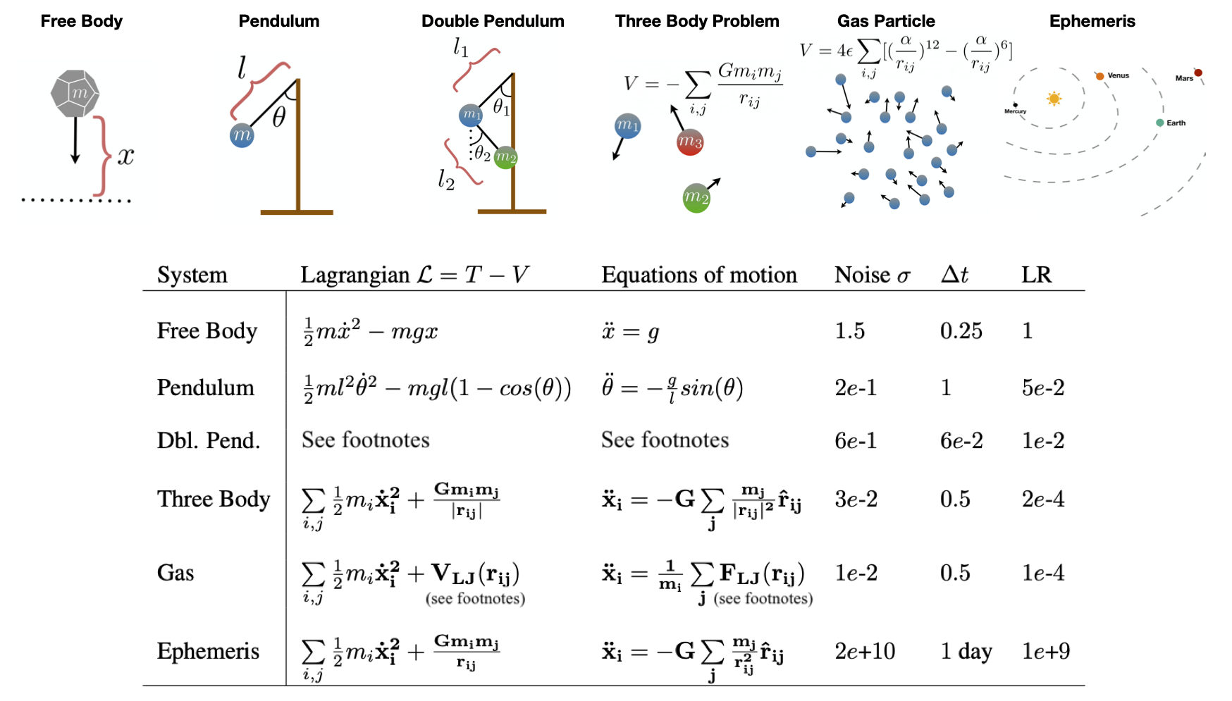
<p>In order to determine how action minimization works on more complex systems, we studied six systems of increasing complexity. The first of these was the free body, which served as a minimal working example, useful for debugging. The next system was a simple pendulum – another minimal working example, but this time with periodic nonlinearities and radial coordinates.</p>

<div class="imgcap" style="display: block; margin-left: auto; margin-right: auto; width:100%;">
  <img src="/assets/ncf/lagn_plus_schema.png" />
</div>

<p>Once we had tuned our approach on these two simple systems, we turned our attention to four more complex systems: a double pendulum, the three body problem, a simple gas, and a real ephemeris dataset of planetary motion (the orbits were projected onto a 2D plane). These systems presented an interesting challenge because they were all nonlinear, chaotic, and high-dimensional.<sup id="fnref:fn0" role="doc-noteref"><a href="#fn:fn0" class="footnote" rel="footnote">1</a></sup> In each case, we compared our results to a baseline path obtained with a simple ODE solver using Euler integration.</p>

<h2 id="the-unconstrained-energy-effect">The unconstrained energy effect</h2>

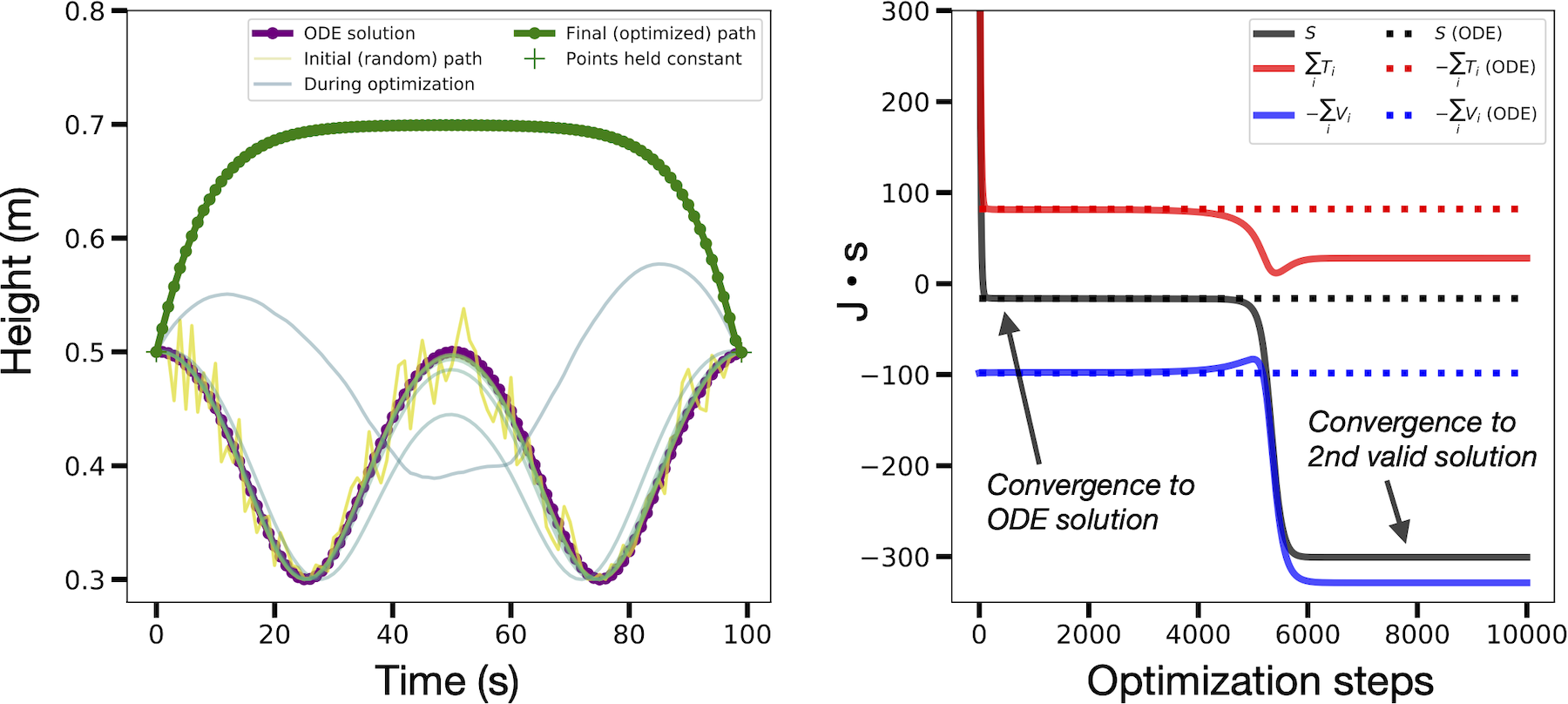
<p>Early in our experiments we encountered <em>the unconstrained energy effect</em>. This happens when the optimizer converges on a valid physical path with a different total energy from the baseline. The figure below shows an example. The reason this happens is that, although we fix the initial and final states, we do not constrain the path’s total energy \(T+V\). Even though paths like the one shown below are not necessarily invalid, they make it difficult for us to recover baseline paths.</p>

<div class="imgcap_noborder" style="display: block; margin-left: auto; margin-right: auto; width:70%;min-width: 300px;">
  <img src="/assets/ncf/unconstrained.png" />
</div>

<p>For this reason, we used the baseline ODE paths to initialize our paths, perturbed them with Gaussian noise, and then used early stopping to select for paths which were similar (often, identical) to the ODE baselines. This approach matched the mathematical ansatz of the “calculus of variations” where one studies perturbed paths in the vicinity of the true path. We note that there are other ways to mitigate this effect which don’t require an ODE-generated initial path.<sup id="fnref:fn1" role="doc-noteref"><a href="#fn:fn1" class="footnote" rel="footnote">2</a></sup></p>

<h2 id="results">Results</h2>

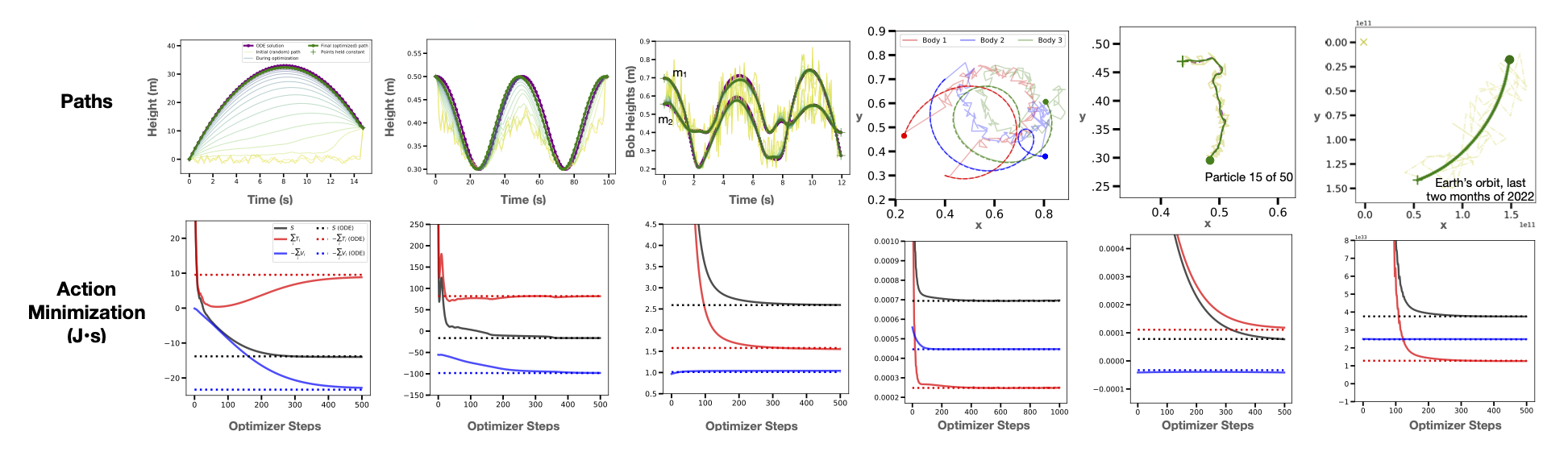
<p>On all six physical systems we obtained paths of least action which were nearly identical to the baseline paths. In the figure below you can also see the optimization dynamics. Our results suggest that action minimization can generate physically-valid dynamics even for chaotic and strongly-coupled systems like the double pendulum and three body problem. One interesting pattern we noticed was that optimization dynamics were dominated by the kinetic energy term \(T\). This occured because \(S\) tended to be more sensitive to \(T\) (which grew as \({\bf \dot{x}}^2\)) than \(V\).</p>

<div class="imgcap" style="display: block; margin-left: auto; margin-right: auto; width:100%;">
  <img src="/assets/ncf/results.png" />
</div>

<h2 id="applications">Applications</h2>

<p>The goal of this post was just to demonstrate that action minimization scales to larger problems. Nevertheless, we can’t help but take a moment to speculate on potential applications of this method:</p>

<ul>
  <li><u>ODE super-resolution.</u> If one were to obtain a low-resolution trajectory via a traditional integration method such as Euler integration, one could then upsample the path by a factor of 10 to 100 (using, eg, linear interpolation) and then run action minimization to make it physically-valid. This procedure would take less time than using the ODE integrator alone.</li>
  <li><u>Infilling missing data.</u> Many real-world datasets have periods of missing data. These might occur due to a sensor malfunction, or they might be built into the experimental setup – for example, a satellite can’t image clouds and weather patterns as well at night – either way, action minimization is well-suited for inferring the sequence of states that connect a fixed start and end state. Doing this with an ODE integrator, meanwhile, is not as natural because there’s no easy way to incorporate the known end state into the problem definition.</li>
  <li><u>When the final state is irrelevant.</u> There are many simulation scenarios where the final state is not important at all. What really matters is that the dynamics look realistic in between times \(t_1\) and \(t_2\). This is the case for simulated smoke in a video game: the smoke just needs to look realistic. With that in mind, we could choose a random final state and then minimize the action of the intervening states. This could allow us to obtain realistic graphics more quickly than numerical methods that don’t fix the final state.</li>
</ul>

<h2 id="discussion">Discussion</h2>

<p>Action minimization shows how the action really does act like a cost function. This isn’t something you’ll hear in your physics courses, even most high-level ones. And yet, it’s an elegant and accurate way to view physics. In a future post, we’ll see how this notion extends even into quantum mechanics.</p>

<h2 id="footnotes">Footnotes</h2>

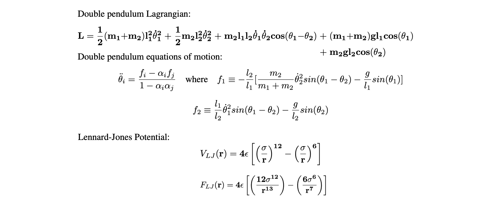
<p>The double pendulum and Lennard-Jones potentials were too long to fit into the table above. Here they are:</p>

<div class="imgcap" style="display: block; margin-left: auto; margin-right: auto; width:100%;">
  <img src="/assets/ncf/lagrangians_fn.png" />
</div>
<div class="footnotes" role="doc-endnotes">
  <ol>
    <li id="fn:fn0" role="doc-endnote">
      <p>The state of the simple gas, for example, has a hundred degrees of freedom. <a href="#fnref:fn0" class="reversefootnote" role="doc-backlink">&#8617;</a></p>
    </li>
    <li id="fn:fn1" role="doc-endnote">
      <p>We discuss these in the Appendix of the paper. <a href="#fnref:fn1" class="reversefootnote" role="doc-backlink">&#8617;</a></p>
    </li>
  </ol>
</div>]]></content><author><name>Sam Greydanus, Tim Strang, and Isabella Caruso</name></author><summary type="html"><![CDATA[Using action minimization, we obtain dynamics for six different physical systems including a double pendulum and a gas with a Lennard-Jones potential.]]></summary></entry><entry><title type="html">Finding Paths of Least Action with Gradient Descent</title><link href="http://greydanus.github.io/2023/03/05/ncf-tutorial/" rel="alternate" type="text/html" title="Finding Paths of Least Action with Gradient Descent" /><published>2023-03-05T12:00:00+00:00</published><updated>2023-03-05T12:00:00+00:00</updated><id>http://greydanus.github.io/2023/03/05/ncf-tutorial</id><content type="html" xml:base="http://greydanus.github.io/2023/03/05/ncf-tutorial/"><![CDATA[<style>
.wrap {
    max-width: 900px;
}
p {
    font-family: sans-serif;
    font-size: 16.75px;
    font-weight: 300;
    overflow-wrap: break-word; /* allow wrapping of very very long strings, like txids */
}
.post pre,
.post code {
    background-color: #fafafa;
    font-size: 14px; /* make code smaller for this post... */
}
pre {
 white-space: pre-wrap;       /* css-3 */
 white-space: -moz-pre-wrap;  /* Mozilla, since 1999 */
 white-space: -pre-wrap;      /* Opera 4-6 */
 white-space: -o-pre-wrap;    /* Opera 7 */
 word-wrap: break-word;       /* Internet Explorer 5.5+ */
}
</style>

<div class="imgcap_noborder" style="display: inline-block; margin-left: auto; margin-right: auto; width:99.9%;margin-bottom: 0px;">
  <div style="width:225px; display: inline-block; vertical-align: top;text-align:center;padding-right:10px;">
    <img alt="" src="/assets/ncf/compare.png" width="95%" id="compareImage" />
    <button id="compareButton" onclick="toggleCompare()" class="playbutton">Play</button>
  </div>
</div>

<p>The purpose of this simple post is to bring to attention a view of physics which isn’t often communicated in introductory courses: the view of <em>physics as optimization</em>.</p>

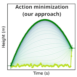
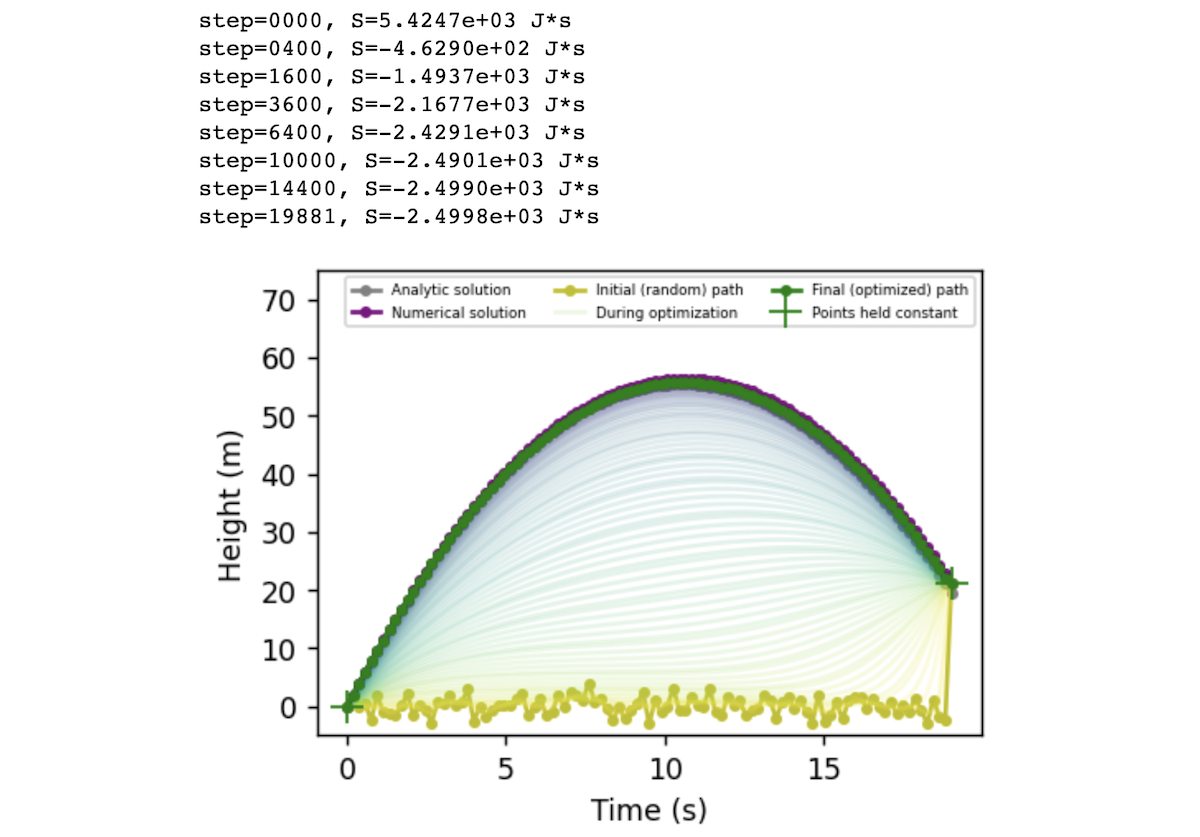
<p>This approach begins with a quantity called the action. If you minimize the action, you can obtain a <em>path of least action</em> which represents the path a physical system will take through space and time. Generally speaking, physicists use analytic tools to do this minimization. In this post, we are going to attempt something different and slightly crazy: minimizing the action with gradient descent.</p>

<div style="display: block; margin-left: auto; margin-right:auto; width:100%; text-align:center;">
  <a href="https://arxiv.org/abs/2303.02115" id="linkbutton" target="_blank">Read the paper</a>
  <a href="https://colab.research.google.com/github/greydanus/ncf/blob/main/tutorial.ipynb" id="linkbutton" target="_blank"><span class="colab-span">Run</span> in browser</a>
  <a href="https://github.com/greydanus/ncf" id="linkbutton" target="_blank">Get the code</a>
</div>

<p><strong>In this post.</strong> In order to communicate this technique as clearly and concretely as possible, we’re going to apply it to a simple toy problem: a free body in a gravitational field. Keep in mind, though, that it works just as well on larger and more complex systems such as an ideal gas – we will treat these sorts of systems in the paper and in future blog posts.</p>

<p>Now, to put our approach in the proper context, we’re going to quickly review the standard approaches to this kind of problem.</p>

<!-- <div class="imgcap" style="display: block; margin-left: auto; margin-right: auto; width:100%">
  <img style='width:51.6%; min-width:330px;' src="/assets/ncf/hero1.png">
  <img style='width:47.5%; min-width:330px;' src="/assets/ncf/hero2.png">
  <div class="thecap"  style="text-align:left;padding-left:0px;">
    We solve a simulation problem as though it were an optimization problem. First we compute the action <i>S</i>, then we minimize it. In doing so, we deform the initial random path (yellow) into the path of least action (blue). The final path happens to be a parabola -- the trajectory that a falling object would take in the real world.
  </div>
</div> -->

<!-- <div class="imgcap_noborder" style="display: block; margin-left: auto; margin-right: auto; width:99.9%">
  <div style="width:100%; min-width:250px; display: inline-block; vertical-align: top;text-align:center;padding-right:10px;">
    <img alt="" src="/assets/ncf/hero.png" width="95%" id="lossImage" />
    <div style="text-align:left;margin-left:10px;margin-right:10px;text-align:center">Caption 2</div>
  </div>
</div> -->

<h3 id="standard-approaches">Standard approaches</h3>

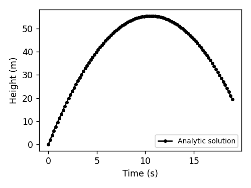
<p><strong>The analytical approach.</strong> Here you use algebra, calculus, and other mathematical tools to find a closed-form equation of motion for the system. It gives the state of the system as a function of time. For an object in free fall, the equation of motion would be:</p>

\[y(t)=-\frac{1}{2}gt^2+v_0t+y_0.\]

<div class="language-python highlighter-rouge"><div class="highlight"><pre class="highlight"><code><span class="k">def</span> <span class="nf">falling_object_analytical</span><span class="p">(</span><span class="n">x0</span><span class="p">,</span> <span class="n">x1</span><span class="p">,</span> <span class="n">dt</span><span class="p">,</span> <span class="n">g</span><span class="o">=</span><span class="mi">1</span><span class="p">,</span> <span class="n">steps</span><span class="o">=</span><span class="mi">100</span><span class="p">):</span>
    <span class="n">v0</span> <span class="o">=</span> <span class="p">(</span><span class="n">x1</span> <span class="o">-</span> <span class="n">x0</span><span class="p">)</span> <span class="o">/</span> <span class="n">dt</span>
    <span class="n">t</span> <span class="o">=</span> <span class="n">np</span><span class="p">.</span><span class="n">linspace</span><span class="p">(</span><span class="mi">0</span><span class="p">,</span> <span class="n">steps</span><span class="p">,</span> <span class="n">steps</span><span class="o">+</span><span class="mi">1</span><span class="p">)</span> <span class="o">*</span> <span class="n">dt</span>
    <span class="n">x</span> <span class="o">=</span> <span class="o">-</span><span class="p">.</span><span class="mi">5</span><span class="o">*</span><span class="n">g</span><span class="o">*</span><span class="n">t</span><span class="o">**</span><span class="mi">2</span> <span class="o">+</span> <span class="n">v0</span><span class="o">*</span><span class="n">t</span> <span class="o">+</span> <span class="n">x0</span>  <span class="c1"># the equation of motion
</span>    <span class="k">return</span> <span class="n">t</span><span class="p">,</span> <span class="n">x</span>

<span class="n">x0</span><span class="p">,</span> <span class="n">x1</span> <span class="o">=</span> <span class="p">[</span><span class="mi">0</span><span class="p">,</span> <span class="mi">2</span><span class="p">]</span>
<span class="n">dt</span> <span class="o">=</span> <span class="mf">0.19</span>
<span class="n">t_ana</span><span class="p">,</span> <span class="n">x_ana</span> <span class="o">=</span> <span class="n">falling_object_analytical</span><span class="p">(</span><span class="n">x0</span><span class="p">,</span> <span class="n">x1</span><span class="p">,</span> <span class="n">dt</span><span class="p">)</span>
</code></pre></div></div>
<div class="imgcap_noborder" style="display: block; margin-left: auto; margin-right: auto; width:300px">
  <img src="/assets/ncf/tutorial_ana.png" />
</div>

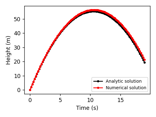
<p><strong>The numerical approach.</strong> Not all physics problems have an analytical solution. Some, like the <a href="https://en.wikipedia.org/wiki/Double_pendulum">double pendulum</a> or the <a href="https://en.wikipedia.org/wiki/Three-body_problem">three-body problem</a>, are deterministic but chaotic. In other words, their dynamics are predictable but we can’t know their state at some time in the future without simulating all the intervening states. These we can solve with numerical integration. For the body in a gravitational field, here’s what the numerical approach would look like:</p>

\[\frac{\partial y}{\partial t} = v(t) \quad \textrm{and} \quad \frac{\partial v}{\partial t} = -g\]

<div class="language-python highlighter-rouge"><div class="highlight"><pre class="highlight"><code><span class="k">def</span> <span class="nf">falling_object_numerical</span><span class="p">(</span><span class="n">x0</span><span class="p">,</span> <span class="n">x1</span><span class="p">,</span> <span class="n">dt</span><span class="p">,</span> <span class="n">g</span><span class="o">=</span><span class="mi">1</span><span class="p">,</span> <span class="n">steps</span><span class="o">=</span><span class="mi">100</span><span class="p">):</span>
    <span class="n">xs</span> <span class="o">=</span> <span class="p">[</span><span class="n">x0</span><span class="p">,</span> <span class="n">x1</span><span class="p">]</span>
    <span class="n">ts</span> <span class="o">=</span> <span class="p">[</span><span class="mi">0</span><span class="p">,</span> <span class="n">dt</span><span class="p">]</span>
    <span class="n">v</span> <span class="o">=</span> <span class="p">(</span><span class="n">x1</span> <span class="o">-</span> <span class="n">x0</span><span class="p">)</span> <span class="o">/</span> <span class="n">dt</span>
    <span class="n">x</span> <span class="o">=</span> <span class="n">xs</span><span class="p">[</span><span class="o">-</span><span class="mi">1</span><span class="p">]</span>
    <span class="k">for</span> <span class="n">i</span> <span class="ow">in</span> <span class="nb">range</span><span class="p">(</span><span class="n">steps</span><span class="o">-</span><span class="mi">1</span><span class="p">):</span>
        <span class="n">v</span> <span class="o">+=</span> <span class="o">-</span><span class="n">g</span><span class="o">*</span><span class="n">dt</span>
        <span class="n">x</span> <span class="o">+=</span> <span class="n">v</span><span class="o">*</span><span class="n">dt</span>
        <span class="n">xs</span><span class="p">.</span><span class="n">append</span><span class="p">(</span><span class="n">x</span><span class="p">)</span>
        <span class="n">ts</span><span class="p">.</span><span class="n">append</span><span class="p">(</span><span class="n">ts</span><span class="p">[</span><span class="o">-</span><span class="mi">1</span><span class="p">]</span><span class="o">+</span><span class="n">dt</span><span class="p">)</span>
    <span class="k">return</span> <span class="n">np</span><span class="p">.</span><span class="n">asarray</span><span class="p">(</span><span class="n">ts</span><span class="p">),</span> <span class="n">np</span><span class="p">.</span><span class="n">asarray</span><span class="p">(</span><span class="n">xs</span><span class="p">)</span>

<span class="n">t_num</span><span class="p">,</span> <span class="n">x_num</span> <span class="o">=</span> <span class="n">falling_object_numerical</span><span class="p">(</span><span class="n">x0</span><span class="p">,</span> <span class="n">x1</span><span class="p">,</span> <span class="n">dt</span><span class="p">)</span>
</code></pre></div></div>
<div class="imgcap_noborder" style="display: block; margin-left: auto; margin-right: auto; width:300px">
  <img src="/assets/ncf/tutorial_num.png" />
</div>

<h3 id="our-approach-action-minimization">Our approach: action minimization</h3>

<p><strong>The Lagrangian method.</strong> The approaches we just covered make intuitive sense. That’s why we teach them in introductory physics classes. But there is an entirely different way of looking at dynamics called the Lagrangian method. The Lagrangian method does a better job of describing reality because it can produce equations of motion for <em>any</em> physical system.<sup id="fnref:fn4" role="doc-noteref"><a href="#fn:fn4" class="footnote" rel="footnote">1</a></sup> Lagrangians figure prominently in all four branches of physics: classical mechanics, electricity and magnetism, thermodynamics, and quantum mechanics. Without the Lagrangian method, physicists would have a hard time unifying these disparate fields. But with the <a href="https://www.symmetrymagazine.org/article/the-deconstructed-standard-model-equation">Standard Model Lagrangian</a> they can do precisely that.</p>

<p><strong>How it works.</strong> The Lagrangian method begins by considering all the paths a physical system could take from an initial state \(\bf{x}\)\((t_0)\) to a final state \(\bf{x}\)\((t_1)\). Then it provides a simple rule for selecting the path \(\hat{\bf x}\) that nature will actually take: the action \(S\), defined in the equation below, must have a stationary value over this path. Here \(T\) and \(V\) are the kinetic and potential energy functions for the system at any given time \(t\) in \([t_0,t_1]\).</p>

\[\begin{aligned}
S &amp;:= \int_{t_0}^{t_1} L({\bf x}, ~ \dot{\bf x}, ~ t) ~ dt\\
&amp;\quad \textrm{where}\quad L = T - V \\
\quad \hat{\bf x} &amp;~~ \textrm{has property}~ \frac{d}{dt} \left( \frac{\partial L}{\partial \dot{\hat{x}}(t)} \right) = \frac{\partial L}{\partial \hat{x}(t)} \\
&amp;\textrm{for} \quad t \in [t_0,t_1]
\end{aligned}\]

<p><strong>Finding \(\hat{\bf x}\) with Euler-Lagrange (what people usually do).</strong> When \(S\) is stationary, we can show that the Euler-Lagrange equation (third line in the equation above) holds true over the interval \([t_0,t_1]\) (Morin, 2008). This observation is valuable because it allows us to solve for \(\hat{\bf x}\): first we apply the Euler-Lagrange equation to the Lagrangian \(L\) and derive a system of partial differential equations.<sup id="fnref:fn3" role="doc-noteref"><a href="#fn:fn3" class="footnote" rel="footnote">2</a></sup> Then we integrate those equations to obtain \(\hat{\bf x}\). Importantly, this approach works for all problems spanning classical mechanics, electrodynamics, thermodynamics, and relativity. It provides a coherent theoretical framework for studying classical physics as a whole.</p>

<p><strong>Finding \(\hat{\bf x}\) with action minimization (what we are going to do).</strong> A more direct approach to finding \(\hat{\bf x}\) begins with the insight that paths of stationary action are almost always <em>also</em> paths of least action (Morin 2008). Thus, without much loss of generality, we can exchange the Euler-Lagrange equation for the simple minimization objective shown in the third line of the equation below. Meanwhile, as shown in the first line, we can redefine \(S\) as a discrete sum over \(N\) evenly-spaced time slices:</p>

\[\begin{aligned}
S &amp;:= \sum_{i=0}^{N} L({\bf x}, ~ \dot{\bf{x}}, ~ t_i) \Delta t \\
 &amp;\textrm{where} \quad \dot{\bf{x}} (t_i) := \frac{ {\bf x}(t_{i+1}) - {\bf x}(t_{i})}{\Delta t} \\
 &amp;\textrm{and} \quad \hat{\bf x} := \underset{\bf x}{\textrm{argmin}} ~ S(\bf x)
\end{aligned}\]

<p>One problem remains: having discretized \( \hat{\bf{x}} \) we can no longer take its derivative to obtain an exact value for \( \dot{\bf{x}}(t_i) \). Instead, we must use the finite-differences approximation shown in the second line. Of course, this approximation will not be possible for the very last \( \dot{\bf{x}} \) in the sum because \(\dot{\bf{x}}_{N+1}\) does not exist. For this value we will assume that, for large \(N\), the change in velocity over the interval \( \Delta t \) is small and thus let \(\dot{\bf{x}}_N = \dot{\bf{x}}_{N-1}\). Having made this last approximation, we can now compute the gradient \(\frac{\partial S}{\partial \bf{x}}\) numerically and use it to minimize \(S\). This can be done with PyTorch (Paszke et al, 2019) or any other package that supports automatic differentiation.</p>

<h3 id="a-simple-implementation">A simple implementation</h3>

<p>Let’s begin with a list of coordinates, <code class="language-plaintext highlighter-rouge">x</code>, which contains all the position coordinates of the system between t\(_1\) and t\(_2\). We can write the Lagrangian and the action of the system in terms of these coordinates.</p>

<div class="language-python highlighter-rouge"><div class="highlight"><pre class="highlight"><code><span class="k">def</span> <span class="nf">lagrangian_freebody</span><span class="p">(</span><span class="n">x</span><span class="p">,</span> <span class="n">xdot</span><span class="p">,</span> <span class="n">m</span><span class="o">=</span><span class="mi">1</span><span class="p">,</span> <span class="n">g</span><span class="o">=</span><span class="mi">1</span><span class="p">):</span>
    <span class="n">T</span> <span class="o">=</span> <span class="p">.</span><span class="mi">5</span><span class="o">*</span><span class="n">m</span><span class="o">*</span><span class="n">xdot</span><span class="o">**</span><span class="mi">2</span>
    <span class="n">V</span> <span class="o">=</span> <span class="n">m</span><span class="o">*</span><span class="n">g</span><span class="o">*</span><span class="n">x</span>
    <span class="k">return</span> <span class="n">T</span><span class="p">,</span> <span class="n">V</span>
  
<span class="k">def</span> <span class="nf">action</span><span class="p">(</span><span class="n">x</span><span class="p">,</span> <span class="n">dt</span><span class="p">):</span>
    <span class="n">xdot</span> <span class="o">=</span> <span class="p">(</span><span class="n">x</span><span class="p">[</span><span class="mi">1</span><span class="p">:]</span> <span class="o">-</span> <span class="n">x</span><span class="p">[:</span><span class="o">-</span><span class="mi">1</span><span class="p">])</span> <span class="o">/</span> <span class="n">dt</span>
    <span class="n">xdot</span> <span class="o">=</span> <span class="n">torch</span><span class="p">.</span><span class="n">cat</span><span class="p">([</span><span class="n">xdot</span><span class="p">,</span> <span class="n">xdot</span><span class="p">[</span><span class="o">-</span><span class="mi">1</span><span class="p">:]],</span> <span class="n">axis</span><span class="o">=</span><span class="mi">0</span><span class="p">)</span>
    <span class="n">T</span><span class="p">,</span> <span class="n">V</span> <span class="o">=</span> <span class="n">lagrangian_freebody</span><span class="p">(</span><span class="n">x</span><span class="p">,</span> <span class="n">xdot</span><span class="p">)</span>
    <span class="k">return</span> <span class="n">T</span><span class="p">.</span><span class="nb">sum</span><span class="p">()</span><span class="o">-</span><span class="n">V</span><span class="p">.</span><span class="nb">sum</span><span class="p">()</span>
</code></pre></div></div>

<p>Now let’s look for a point of stationary action. Technically, this could be a minimum OR an inflection point.<sup id="fnref:fn1" role="doc-noteref"><a href="#fn:fn1" class="footnote" rel="footnote">3</a></sup> Here, we’re just going to look for a minimum:</p>

<div class="language-python highlighter-rouge"><div class="highlight"><pre class="highlight"><code><span class="k">def</span> <span class="nf">get_path_between</span><span class="p">(</span><span class="n">x</span><span class="p">,</span> <span class="n">steps</span><span class="o">=</span><span class="mi">1000</span><span class="p">,</span> <span class="n">step_size</span><span class="o">=</span><span class="mf">1e-1</span><span class="p">,</span> <span class="n">dt</span><span class="o">=</span><span class="mi">1</span><span class="p">,</span> <span class="n">num_prints</span><span class="o">=</span><span class="mi">15</span><span class="p">,</span> <span class="n">num_stashes</span><span class="o">=</span><span class="mi">80</span><span class="p">):</span>
    <span class="n">t</span> <span class="o">=</span> <span class="n">np</span><span class="p">.</span><span class="n">linspace</span><span class="p">(</span><span class="mi">0</span><span class="p">,</span> <span class="nb">len</span><span class="p">(</span><span class="n">x</span><span class="p">)</span><span class="o">-</span><span class="mi">1</span><span class="p">,</span> <span class="nb">len</span><span class="p">(</span><span class="n">x</span><span class="p">))</span> <span class="o">*</span> <span class="n">dt</span>
    <span class="n">print_on</span> <span class="o">=</span> <span class="n">np</span><span class="p">.</span><span class="n">linspace</span><span class="p">(</span><span class="mi">0</span><span class="p">,</span><span class="nb">int</span><span class="p">(</span><span class="n">np</span><span class="p">.</span><span class="n">sqrt</span><span class="p">(</span><span class="n">steps</span><span class="p">)),</span><span class="n">num_prints</span><span class="p">).</span><span class="n">astype</span><span class="p">(</span><span class="n">np</span><span class="p">.</span><span class="n">int32</span><span class="p">)</span><span class="o">**</span><span class="mi">2</span> <span class="c1"># print more early on
</span>    <span class="n">stash_on</span> <span class="o">=</span> <span class="n">np</span><span class="p">.</span><span class="n">linspace</span><span class="p">(</span><span class="mi">0</span><span class="p">,</span><span class="nb">int</span><span class="p">(</span><span class="n">np</span><span class="p">.</span><span class="n">sqrt</span><span class="p">(</span><span class="n">steps</span><span class="p">)),</span><span class="n">num_stashes</span><span class="p">).</span><span class="n">astype</span><span class="p">(</span><span class="n">np</span><span class="p">.</span><span class="n">int32</span><span class="p">)</span><span class="o">**</span><span class="mi">2</span>
    <span class="n">xs</span> <span class="o">=</span> <span class="p">[]</span>
    <span class="k">for</span> <span class="n">i</span> <span class="ow">in</span> <span class="nb">range</span><span class="p">(</span><span class="n">steps</span><span class="p">):</span>
        <span class="n">grad_x</span> <span class="o">=</span> <span class="n">torch</span><span class="p">.</span><span class="n">autograd</span><span class="p">.</span><span class="n">grad</span><span class="p">(</span><span class="n">action</span><span class="p">(</span><span class="n">x</span><span class="p">,</span> <span class="n">dt</span><span class="p">),</span> <span class="n">x</span><span class="p">)[</span><span class="mi">0</span><span class="p">]</span>
        <span class="n">grad_x</span><span class="p">[[</span><span class="mi">0</span><span class="p">,</span><span class="o">-</span><span class="mi">1</span><span class="p">]]</span> <span class="o">*=</span> <span class="mi">0</span>  <span class="c1"># fix first and last coordinates by zeroing their gradients
</span>        <span class="n">x</span><span class="p">.</span><span class="n">data</span> <span class="o">-=</span> <span class="n">grad_x</span> <span class="o">*</span> <span class="n">step_size</span>

        <span class="k">if</span> <span class="n">i</span> <span class="ow">in</span> <span class="n">print_on</span><span class="p">:</span>
            <span class="k">print</span><span class="p">(</span><span class="s">'step={:04d}, S={:.4e}'</span><span class="p">.</span><span class="nb">format</span><span class="p">(</span><span class="n">i</span><span class="p">,</span> <span class="n">action</span><span class="p">(</span><span class="n">x</span><span class="p">,</span> <span class="n">dt</span><span class="p">).</span><span class="n">item</span><span class="p">()))</span>
        <span class="k">if</span> <span class="n">i</span> <span class="ow">in</span> <span class="n">stash_on</span><span class="p">:</span>
            <span class="n">xs</span><span class="p">.</span><span class="n">append</span><span class="p">(</span><span class="n">x</span><span class="p">.</span><span class="n">clone</span><span class="p">().</span><span class="n">data</span><span class="p">.</span><span class="n">numpy</span><span class="p">())</span>
    <span class="k">return</span> <span class="n">t</span><span class="p">,</span> <span class="n">x</span><span class="p">,</span> <span class="n">np</span><span class="p">.</span><span class="n">stack</span><span class="p">(</span><span class="n">xs</span><span class="p">)</span>
</code></pre></div></div>

<p>Now let’s put it all together. We can initialize our falling particle’s path to be any random path through space. In the code below, we choose a path where the particle bounces around x=0 at random until time t=19 seconds, at which point it leaps up to its final state of x = <code class="language-plaintext highlighter-rouge">x_num[-1]</code> = 21.3 meters. This path has a high action of S = 5425 J·s. As we run the optimization, this value decreases smoothly until we converge on a parabolic arc with an action of S = -2500 J·s.</p>

<div class="language-python highlighter-rouge"><div class="highlight"><pre class="highlight"><code><span class="n">dt</span> <span class="o">=</span> <span class="mf">0.19</span>
<span class="n">x0</span> <span class="o">=</span> <span class="mf">1.5</span><span class="o">*</span><span class="n">torch</span><span class="p">.</span><span class="n">randn</span><span class="p">(</span><span class="nb">len</span><span class="p">(</span><span class="n">x_num</span><span class="p">),</span> <span class="n">requires_grad</span><span class="o">=</span><span class="bp">True</span><span class="p">)</span>  <span class="c1"># a random path through space
</span><span class="n">x0</span><span class="p">[</span><span class="mi">0</span><span class="p">].</span><span class="n">data</span> <span class="o">*=</span> <span class="mf">0.0</span> <span class="p">;</span> <span class="n">x0</span><span class="p">[</span><span class="o">-</span><span class="mi">1</span><span class="p">].</span><span class="n">data</span> <span class="o">*=</span> <span class="mf">0.0</span>  <span class="c1"># set first and last points to zero
</span><span class="n">x0</span><span class="p">[</span><span class="o">-</span><span class="mi">1</span><span class="p">].</span><span class="n">data</span> <span class="o">+=</span> <span class="n">x_num</span><span class="p">[</span><span class="o">-</span><span class="mi">1</span><span class="p">]</span>  <span class="c1"># set last point to be the end height of the numerical solution
</span>
<span class="n">t</span><span class="p">,</span> <span class="n">x</span><span class="p">,</span> <span class="n">xs</span> <span class="o">=</span> <span class="n">get_path_between</span><span class="p">(</span><span class="n">x0</span><span class="p">.</span><span class="n">clone</span><span class="p">(),</span> <span class="n">steps</span><span class="o">=</span><span class="mi">20000</span><span class="p">,</span> <span class="n">step_size</span><span class="o">=</span><span class="mf">1e-2</span><span class="p">,</span> <span class="n">dt</span><span class="o">=</span><span class="n">dt</span><span class="p">)</span>
</code></pre></div></div>

<div class="imgcap_noborder" style="display: block; margin-left: auto; margin-right: auto; width:60%; min-width:330px;">
  <img src="/assets/ncf/tutorial_printout.png" />
</div>

<h3 id="direct-comparison-between-the-numerical-ode-solution-and-our-approach">Direct comparison between the numerical (ODE) solution and our approach</h3>

<p>On the left side of the figure below, we compare the normal approach of ODE integration to our approach of action minimization. As a reminder, the action is the sum, over every point in the path, of kinetic energy \(T\) minus potential energy \(V\). We compute the gradients of this quantity with respect to the path coordinates and then deform the initial path (yellow) into the path of least action (green). This path resolves to a parabola, matching the path obtained via ODE integration. On the right side of the figure, we plot the path’s action \(S\), kinetic energy \(T\), and potential energy \(V\) over the course of optimization. All three quantities asymptote at the respective values of the ODE trajectory.</p>

<div class="imgcap_noborder" style="display: block; margin-left: auto; margin-right: auto; width:100%">
  <img src="/assets/ncf/hero.png" />
</div>

<h3 id="closing-thoughts">Closing thoughts</h3>

<p>As if by snake-charming magic, we have coaxed a path of random coordinates to make a serpentine transition into a structured and orderly parabolic shape – the shape of the one trajectory that a free body will take under the influence of a constant gravitational field. This is a simple example, but we have investigated it in detail because it is illustrative of the broader “principle of least action” which defies natural human intuition and sculpts the very structure of our physical universe.</p>

<p>By the vagueness of its name alone, “the action,” you may sense that it is not a well-understood phenomenon. In subsequent posts, we will explore how it works in more complex classical simulations and then, later, in the realm of quantum mechanics. And after that, we will talk about its history: how it was discovered and what its discoverers thought when they found it. And most importantly, we will address <em>the lingering speculations as to what, exactly, it means</em>.</p>

<!-- The goal of this post was just to demonstrate that it's possible to find a path of least action via gradient descent. Determining whether it has useful applications is a question for another day. Nevertheless, here are a few speculations as to what those applications might look like:

* <u>ODE super-resolution.</u>

* <u>Infilling missing data.</u> Some chaotic deterministic systems

* <u>When the final state is irrelevant.</u> There are many simulation scenarios where the final state is not important at all. What really matters is that the dynamics look realistic in between times t\\(_1\\) and t\\(_2\\). This is the case for simulated smoke in a video game: the smoke just needs to look realistic. With that in mind, we could choose a random final state and then minimize the action of the intervening states. This could allow us to obtain realistic graphics more quickly than numerical methods that don't fix the final state.

The thing I like most about this little experiment is that it shows how the action really does act like a cost function. This isn't something you'll hear in your physics courses, even high level ones. And yet, it's quite surprising and interesting to learn that nature has a cost function! The action is a very, very fundamental quantity. In a future post, we'll see how this notion extends even into quantum mechanics - with a few modifications of course. -->

<!-- Basic physical principles and the elegant reasoning behind them are often obscured in the midst of numerical approximations and domain-specific notation. This post shows that it's surprisingly easy to solve physics by working directly in terms of the action. It lets us solve simulation problems as though they are optimization problems -- a surprising result! -->

<h2 id="footnotes">Footnotes</h2>

<script language="javascript">
  function toggleCompare() {

    path = document.getElementById("compareImage").src
      if (path.split('/').pop() == "compare.png")
      {
          document.getElementById("compareImage").src = "/assets/ncf/compare.gif";
          document.getElementById("compareButton").textContent = "Reset";
      }
      else 
      {
          document.getElementById("compareImage").src = "/assets/ncf/compare.png";
          document.getElementById("compareButton").textContent = "Play";
      }
  }
</script>

<div class="footnotes" role="doc-endnotes">
  <ol>
    <li id="fn:fn4" role="doc-endnote">
      <p>Tim informs me that there are some string theories that can’t be lagranged. So in the interest of precision, I will narrow this claim to cover <em>all physical systems that have been observed experimentally</em>. <a href="#fnref:fn4" class="reversefootnote" role="doc-backlink">&#8617;</a></p>
    </li>
    <li id="fn:fn3" role="doc-endnote">
      <p>See <a href="https://scholar.harvard.edu/files/david-morin/files/cmchap6.pdf">Morin, 2008</a> for an example. <a href="#fnref:fn3" class="reversefootnote" role="doc-backlink">&#8617;</a></p>
    </li>
    <li id="fn:fn1" role="doc-endnote">
      <p>That’s why the whole method is often called <em>The Principle of Least Action</em>, a misnomer which I (and others) have picked up by reading the Feynman lectures. <a href="#fnref:fn1" class="reversefootnote" role="doc-backlink">&#8617;</a></p>
    </li>
  </ol>
</div>]]></content><author><name>Sam Greydanus, Tim Strang, and Isabella Caruso</name></author><summary type="html"><![CDATA[The purpose of this simple post is to bring to attention a view of physics which isn’t often communicated in intro courses: the view of physics as optimization.]]></summary></entry><entry><title type="html">Studying Growth with Neural Cellular Automata</title><link href="http://greydanus.github.io/2022/05/24/studying-growth/" rel="alternate" type="text/html" title="Studying Growth with Neural Cellular Automata" /><published>2022-05-24T06:50:00+00:00</published><updated>2022-05-24T06:50:00+00:00</updated><id>http://greydanus.github.io/2022/05/24/studying-growth</id><content type="html" xml:base="http://greydanus.github.io/2022/05/24/studying-growth/"><![CDATA[<!-- "We simulate the process of cell growth called morphogenesis. Then we find growth rules that generate a range of flowers and use them to grow a garden." -->

<div class="imgcap" style="display: block; margin-left: auto; margin-right: auto; width:99.9%">
  <div style="width:32%; min-width:250px; display: inline-block; vertical-align: top;text-align:center;padding-right:10px;">
    <video id="video1" style="width:100%;min-width:250px;" poster="/assets/studying-growth/rose.jpg">
      <source src="/assets/studying-growth/rose.mp4" type="video/mp4" />
    </video>
    <button class="playbutton" id="video1_button" onclick="playPauseVideo1()">Play</button>
  </div>
  <div style="width:32%; min-width:250px; display: inline-block; vertical-align: top;text-align:center;padding-right:10px;">
    <video id="video2" style="width:100%;min-width:250px;" poster="/assets/studying-growth/marigold.jpg">
      <source src="/assets/studying-growth/marigold.mp4" type="video/mp4" />
    </video>
    <button class="playbutton" id="video2_button" onclick="playPauseVideo2()">Play</button>
  </div>
   <div style="width:32%; min-width:250px; display: inline-block; vertical-align: top;text-align:center;">
    <video id="video3" style="width:100%;min-width:250px;" poster="/assets/studying-growth/crocus.jpg">
      <source src="/assets/studying-growth/crocus.mp4" type="video/mp4" />
    </video>
    <button class="playbutton" id="video3_button" onclick="playPauseVideo3()">Play</button>
  </div>
  <div style="text-align:left; display:block; margin-left: auto; margin-right: auto; width:95%"><b>Growing flowers.</b> The pixels in the images above represent cells. By exchanging signals with their neighbors, these cells coordinate their behavior and assemble themselves in the shapes of the three flowers shown.</div>
</div>

<script> 
function playPauseVideo1() { 
  var video = document.getElementById("video1"); 
  var button = document.getElementById("video1_button");
  if (video.paused) {
    video.play();
    button.textContent = "Pause";}
  else {
    video.pause(); 
  button.textContent = "Play";}
} 

function playPauseVideo2() { 
  var video = document.getElementById("video2"); 
  var button = document.getElementById("video2_button");
  if (video.paused) {
    video.play();
  button.textContent = "Pause";}
  else {
    video.pause(); 
  button.textContent = "Play";}
} 

function playPauseVideo3() { 
  var video = document.getElementById("video3"); 
  var button = document.getElementById("video3_button");
  if (video.paused) {
    video.play();
  button.textContent = "Pause";}
  else {
    video.pause(); 
  button.textContent = "Play";}
} 
</script>

<div style="display: block; margin-left: auto; margin-right: auto; width:100%; text-align:center;">
  <a href="https://colab.research.google.com/drive/1TgGN5qjjH6MrMrTcStEkdHO-giEJ4bZr" id="linkbutton" target="_blank"><span class="colab-span">Run</span> in browser</a>
  <a href="https://github.com/greydanus/studying_growth" id="linkbutton" target="_blank">Get the code</a>
</div>

<!-- ## A Productive Question -->

<p>How does a single fertilized egg grow into a population of seventy trillion cells: a population that can walk, talk, and write sonnets? This is one of the great unanswered questions of biology. We may never finish answering it, but it is a productive question nonetheless. In asking it, scientists have discovered the structure of DNA, sequenced the human genome, and made essential contributions to modern medicine.</p>

<p>In this post, we will explore this question with a new tool called Neural Cellular Automata (NCA).</p>

<!-- **Neural Cellular Automata.** A few years ago, scientists showed that it is possible to use neural networks to represent the rules for how simulated cells interact with one another. This allowed them to teach simulated cells to interact with one another at a local scale in order to produce complex emergent behaviors at the population level. So far, only a few papers have been written about these "Neural Cellular Automata" models. One reason is that they are a relatively new idea. Another reason is that, although they require expertise in ML to implement, their main intellectual appeal is to an audience interested in cellular morphogenesis. The intersection of people who are comfortable in both worlds is relatively small.

But the mechanics of cellular morphogenesis are extremely important. Indeed, NCA may be the best long-term means of understanding the programming language of our bodies' cells. If DNA is the source code that comes pre-installed on your computer, then cellular morphogenesis is the complex and varied means by which your computer performs its functions: booting up, decompressing files, creating pop-up windows, and so forth. In order to understand your computer as a whole, it makes a lot of sense to start by studying the mechanics of these everyday functions.

With all of this in mind, let's take a closer look at how NCA work and then apply them to some simple biology problems. -->

<h2 id="motivation">Motivation</h2>

<p>The purpose of cellular automata (CA) <em>writ large</em> is to mimic biological growth at the cellular level. Most CAs begin with a grid of pixels where each pixel represents a different cell. Then a set of growth rules, controlling how cells respond to their neighbors, are applied to the population in an iterative manner. Although these growth rules are simple to write down, they are choosen so as to produce complex self-organizing behaviors. For example, Conway’s Game of Life has just three simple growth rules that give rise to a diverse range of structures.<sup id="fnref:fn4" role="doc-noteref"><a href="#fn:fn4" class="footnote" rel="footnote">1</a></sup></p>

<div class="imgcap" style="display: block; margin-left: auto; margin-right: auto; width:99.9%">
  <div style="width:49.4%; min-width:280px; display: inline-block; vertical-align: top;text-align:center;">
    <img src="/assets/studying-growth/conway_rules.jpg" />
  </div>
  <div style="width:49.7%; min-width:280px; display: inline-block; vertical-align: top;text-align:center;">
    <video id="video_conway" controls="" style="width:100%">
      <source src="/assets/studying-growth/conway.mp4" type="video/mp4" />
    </video>
  </div>
</div>

<p>Classic versions of cellular automata like Conway’s Game of Life are interesting because they produce emergent behavior starting from simple rules. But in a way, these versions of CA are <em>too simple</em>. Their cells only get to have two states, dead or alive, whereas biological cells get to have a near-infinite number of states, states which are determined by a wide variety of signaling molecules. We refer to these molecules as <em>morphogens</em> because they work together to control growth and guide organisms towards specific final shapes or <em>morphologies</em>.</p>

<p><strong>Neural CA.</strong> Based on this observation, we should move away from CA with cells that are only dead or alive. Instead, we should permit their cells to exist in a variety of states with each state defined by a list of continuous variables. Growth rules should operate on combinations of these variables in the same way that biological growth rules operate on combinations of different morphogens. And unlike Conway’s Game of Life, the self-organizing behaviors that arise should not be arbitrary or chaotic. Rather, they should involve stable convergence to <em>specific</em> large-scale morphologies like those that occur in biology. Much more complex growth rules are needed for this to occur.</p>

<div class="imgcap_noborder" style="display: block; margin-left: auto; margin-right: auto; width:100%">
  <img src="/assets/studying-growth/comparison.jpg" />
</div>

<p>The diagram above shows how NCA take a step in the right direction. Unlike regular cellular automata, they represent each cell state with a real-valued \(n\)-dimensional vector and then allow arbitrary growth rules to operate on that domain. They do this by <em>parameterizing growth rules with a neural network and then optimizing the neural network to obtain the desired pattern of growth</em>. To showcase the model’s expressivity, the authors trained it to arrange a population of a 1600 cells in the shape of a lizard starting from local-only interactions between initially identical cells.</p>

<div class="imgcap_noborder" style="display: block; margin-left: auto; margin-right: auto; width:100%">
  <img src="/assets/studying-growth/nca_schema.jpg" />
  <div class="thecap" style="text-align:left; display:block; margin-left: auto; margin-right: auto; width:100%">
  <b>NCA diagram.</b> The diagram above how a neural network can be used to parameterize the growth rules of a cellular autiomata. The <a href="https://distill.pub/2020/growing-ca/">original NCA article</a> uses this diagram to introduce the model and its training procedure.
  </div>
</div>

<h2 id="getting-started">Getting started</h2>

<!-- We need to start with a high-quality NCA implementation, one that is flexible enough to modify for the purposes of our experiments. The authors of the original NCA paper released a series of excellent Colab notebooks which show how to implement the model in TensorFlow. But after experimenting with their code, I decided to reimplement everything in PyTorch. I like PyTorch better and I wanted to make a minimalist implementation that would be easy to hack on in order to try out new ideas. You can find it [here](https://colab.research.google.com/drive/13wCM9OV2JR004zFvh7zPgUxrga8sU4d1). -->

<p>The authors of the original paper released a Colab notebook that showed how to implement NCA in TensorFlow. Starting from this notebook, we reimplemented everything in PyTorch and boiled it down to a minimalist, 150-line implementation. Our goal was to make the NCA model as simple as possible so that we could hack and modify it without getting overwhelmed by implementation details.</p>

<div style="display: block; margin-left: auto; margin-right: auto; width:100%; text-align:center;">
  <a href="https://colab.research.google.com/drive/13wCM9OV2JR004zFvh7zPgUxrga8sU4d1" id="linkbutton" target="_blank"><span class="colab-span">NCA</span> in 150 lines</a>
</div>

<p>Having implemented our own NCA model, the next step was to scale it to determine the maximum size and complexity of the “organisms” it could produce. We found that the population size was going to be limited by the amount of RAM available on Google Colab GPUs. We maxed things out with a population of about 7500 cells running for about 100 updates. For context, the original paper used a population of 1600 cells running for 86 updates.</p>

<div class="imgcap_noborder" style="display: block; margin-left: auto; margin-right: auto; width:100%">
  <img src="/assets/studying-growth/bloopers.jpg" />
</div>

<p>Working in this scaled-up regime, we trained our NCA to grow a number of different flowers. Some of the early results were a bit mangled and blurry. Many were biased towards radial symmetry and required extra training in order to reveal symmetric features such as individual petals. But soon, after a few hyperparameter fixes, our NCA was able to grow some “HD” 64x64 flowers:</p>

<div class="imgcap_noborder" style="display: block; margin-left: auto; margin-right: auto; width:65%">
  <img src="/assets/studying-growth/garden.jpg" />
</div>

<div style="display: block; margin-left: auto; margin-right: auto; width:100%; text-align:center;">
  <a href="https://colab.research.google.com/drive/1TgGN5qjjH6MrMrTcStEkdHO-giEJ4bZr" id="linkbutton" target="_blank"><span class="colab-span">HD</span> flowers</a>
</div>

<p>Having implemented the NCA model and gained some intuition for how it trained, we were ready to use it to investigate patterns of biological growth.</p>

<h2 id="patterns-of-biological-growth">Patterns of biological growth</h2>

<p>Biological growth is wonderfully diverse. Consider this passage from the first chapter of <em>Growth</em> by Life Science Library:</p>

<p><em>A eucalyptus native to Uganda has been known to grow 45 feet in two years, whereas dwarf ivy generally grows one inch a year. The majestic sequoia of California, which starts out as a seed weighing only one three-thousandth of an ounce, may end up… [with a] weight estimated at 6,200 tons. It takes more than 1,000 years for the sequoia to achieve the feat of multiplying 600 billion times in mass.</em></p>

<p><em>The animal kingdom, too, has its champions of growth. The blue whale, which cruises the oceans from the North to the South Pole, begins life as a barely visible egg weighing only a fraction of an ounce. At birth, it weighs from two to three tons. When it is weaned, at about seven months, it is 52 feet long and weighs 23 tons, having gained an average of 200 pounds a day.</em></p>

<p>Given the diversity of life forms on our planet, maybe one of the biggest surprises is how much they have in common. For the most part they share the same genetic materials, signaling mechanisms, and metabolic pathways. Their cells have the same life cycles. Indeed, the cellular mechanics in a gnat look pretty similar to those in a blue whale…even though the creatures themselves could not be more different.</p>

<h3 id="1-gnomonic-growth"><a href="https://colab.research.google.com/drive/1DUFL5glyej725r8VAYDZIFrWvpR6a6-0">1. Gnomonic growth</a></h3>

<p>One shared pattern of growth is called <em>gnomonic growth</em>. This pattern tends to occur when an organism needs to increase in size and part of its body is defined by a rigid structure. You can see this in clams, for example. Their shells are rigid and cannot be deformed. And yet they need to grow their shells as the rest of them grows. Clams solve this problem by incrementally adding long crescent-shaped lips to the edges of their shells. Each new lip is just a little larger than the one that came before it. These lips, or <em>gnomons</em> as they are called, permit organisms to increase in size without changing form. Gnomons also appear in horns, tusks, and tree trunks.</p>

<div class="imgcap_noborder" style="display: block; margin-left: auto; margin-right: auto; width:100%; min-width:300px">
  <img src="/assets/studying-growth/gnomons.jpeg" />
</div>

<p>One of the most famous products of gnomonic growth is the nautilus shell. In this shell, the gnomons grow with such regularity that the overall shape can be modeled with a simple Fibonacci sequence. The elegance and simplicity of the pattern makes it an interesting testbed for NCA.</p>

<div class="imgcap_noborder" style="display: block; margin-left: auto; margin-right: auto; width:100%; min-width:300px">
  <img src="/assets/studying-growth/nautilus_photo.jpeg" />
</div>

<p>To set up this problem, we split the shell into three regions: frozen, mature, and growing. These regions are shown in cyan, black and magenta respectively:</p>
<div class="imgcap_noborder" style="display: block; margin-left: auto; margin-right: auto; width:100%">
  <img src="/assets/studying-growth/nautilus_train.png" />
</div>
<p>The cells in the frozen region are, as the name would suggest, frozen. Both their RGBA and hidden channels are fixed throughout training. The cells in the mature region are similar; the only difference is that their hidden channels are allowed to change. The growing region, meanwhile, begins the simulation without any living cells. Cells from the mature region need to grow outwards into this area and arrange themselves properly before the simulation ends.</p>

<p><strong>Scale and rotation invariance.</strong> Part of the objective in this “gnomonic growth” problem is to learn a growth rule that is scale and rotation invariant. We can accomplish this by rotating and scaling the nautilus template as shown in the six examples above. By training on all of these examples at once, we are able to obtain a model that grows properly at any scale or orientation. Once it learns to do this, it can grow multiple gnomons, one after the other, without much interference. Below, for example, we add eight new compartments and quadruple the shell’s size by letting the NCA run for eight growth cycles.<sup id="fnref:fn3" role="doc-noteref"><a href="#fn:fn3" class="footnote" rel="footnote">2</a></sup></p>

<div class="imgcap_noborder" style="display: block; margin-left: auto; margin-right: auto; width:100%">
  <img src="/assets/studying-growth/nautilus_bw.png" />
</div>

<p>One of the things that makes this growth pattern interesting is that the NCA cells have to reach a global consensus as to what the scale and rotation of the mature region is. Only by agreeing on this are they able to construct a properly-sized addition. And yet in practice, we see that expansion into the growth region begins from the first simulation step. This suggests that cells in the mature region try to come to a distributed consensus as to the target shape <em>even as</em> new cells are already beginning to grow that shape. Once cells in the mature region know the proper scale and rotation of the gnomon, they transmit this information to the growing region so that it can make small adjustments to its borders. If you look closely, you can see these adjustments happening in the video below.</p>

<div class="imgcap" style="display: block; margin-left: auto; margin-right: auto; width:99.9%">
  <div style="width:32%; min-width:250px; display: inline-block; vertical-align: top;text-align:center;padding-right:10px;">
    <video id="naut_video" style="width:100%;min-width:250px;" poster="/assets/studying-growth/nautilus.png">
      <source src="/assets/studying-growth/nautilus.mp4" type="video/mp4" />
    </video>
    <button class="playbutton" id="naut_video_button" onclick="playPauseNaut()">Play</button>
  </div>
</div>

<script> 
function playPauseNaut() { 
  var video = document.getElementById("naut_video"); 
  var button = document.getElementById("naut_video_button");
  if (video.paused) {
    video.play();
    button.textContent = "Pause";}
  else {
    video.pause(); 
  button.textContent = "Play";}
} 
</script>

<div style="display: block; margin-left: auto; margin-right: auto; width:100%; text-align:center;">
  <a href="https://colab.research.google.com/drive/1DUFL5glyej725r8VAYDZIFrWvpR6a6-0" id="linkbutton" target="_blank"><span class="colab-span">Growing</span> a nautilus</a>
</div>

<p>This process of <em>reaching a consensus in a decentralized and asynchronous manner</em> is a common problem for biological cells. In fact, we already touched on it in our <a href="/2020/08/27/selforg-mnist/">Self-classifying MNIST Digits</a> post. It’s also important in human organizations: from new cities agreeing on development codes, to democratic institutions agreeing on legislation, to the stock market agreeing on how to value companies. It is not always a low-entropy process.</p>

<p>Indeed, sometimes groups of cells have to resort to other means of reaching consensus…</p>

<h3 id="2-embryonic-induction"><a href="https://colab.research.google.com/drive/1fbakmrgkk1y-ZXamH1mKbN1tvkogNrWq">2. Embryonic induction</a></h3>

<p>The alternative to a fully decentralized consensus mechanism is cellular induction. This happens when one small group of cells (usually in an embryo) tells the rest how to grow. The first group of cells is called the inducing tissue and the second is called the responding tissue. Induction controls the growth of many tissues and organs including the eye and the heart.</p>

<p>In this section, we will grow an image of a newt and then graft part of its eye tissue onto its belly. After doing this, we will watch to see whether those cells are able to induce growth in the rest of the eye in that region. We’ve chosen this particular experiment as an homage to <a href="https://en.wikipedia.org/wiki/Hans_Spemann">Hans Spemann</a>,<sup id="fnref:fn2" role="doc-noteref"><a href="#fn:fn2" class="footnote" rel="footnote">3</a></sup> who won the Nobel Prize for Medicine in 1935 for using similar experiments on real newts to discover “the organizer effect in embryonic development.”<sup id="fnref:fn5" role="doc-noteref"><a href="#fn:fn5" class="footnote" rel="footnote">4</a></sup> Spemann’s major insight was that “at every stage of embryonic development, structures already present act as organizers, inducing the emergence of whatever structures are next on the timetable.”<sup id="fnref:fn7" role="doc-noteref"><a href="#fn:fn7" class="footnote" rel="footnote">5</a></sup></p>

<div class="imgcap_noborder" style="display: block; margin-left: auto; margin-right: auto; width:90%">
  <img src="/assets/studying-growth/newt_timeline_tall.png" style="width:75%; min-width:320px" />
  <!-- <div class="thecap"  style="text-align:left; display:block; margin-left: auto; margin-right: auto; width:100%">
    <b>Reproducing Hans Spemann's newt experiment.</b> In the first 100 frames, we grow an image of a newt using the vanilla NCA model described in <a href="https://distill.pub/2020/growing-ca/">Mordvintsev et al. (2020)</a>. Then, in frame 150 we copy the pixels in the yellow rectangle and paste them onto the newt's belly, as shown by the yellow arrow. Note that these pixels contain the upper half of the newt's eye, but not the lower half. We freeze those cells and let the rest of the cells perform updates for another 25 steps. As you can see in frame 175, this induces the belly cells in the blue rectangle to turn black, completing the lower half of the new eye.
  </div> -->
</div>

<p>To reproduce this effect, we first trained an NCA to grow a picture of a newt. Once the growth phase was complete, we grafted a patch of cells from its head onto its stomach. This patch of cells included the upper, light-colored portion of the newt’s eye but not the dark-colored, lower portion. Then we froze their states and allowed the rest of the cells to undergo updates as usual. Within 25 steps, the stomach cells below the grafted patch had regrown into a dark-colored strip to complete the lower half of the new eye.</p>

<!-- Hans Spemann's experiment involved the same procedure and produced the same results: he grafted eye lens cells onto the stomach of a real newt and induced the growth of a new eye.
 -->
<div class="imgcap" style="display: block; margin-left: auto; margin-right: auto; width:99.9%">
  <div style="width:300px; min-width:250px; display: inline-block; vertical-align: top;text-align:center;">
    <video id="newt_video" style="width:100%;min-width:250px;" controls="" poster="/assets/studying-growth/newt.jpg">
      <source src="/assets/studying-growth/newt.mp4" type="video/mp4" />
    </video>
    <button class="playbutton" id="newt_video_button" onclick="playPauseNewt()">Play</button>
  </div>
</div>

<script> 
function playPauseNewt() { 
  var video = document.getElementById("newt_video"); 
  var button = document.getElementById("newt_video_button");
  if (video.paused) {
    video.play();
    button.textContent = "Pause";}
  else {
    video.pause(); 
  button.textContent = "Play";}
} 
</script>

<div style="display: block; margin-left: auto; margin-right: auto; width:100%; text-align:center;">
  <a href="https://colab.research.google.com/drive/1fbakmrgkk1y-ZXamH1mKbN1tvkogNrWq" id="linkbutton" target="_blank"><span class="colab-span">Embryonic</span> induction</a>
</div>

<p>Cellular induction offers a simple explanation for how many growth rules are implemented: by and large, they are implemented as <code>if-then</code> statements. For example, <em>“If I am growing below some light-colored eye tissue, then I should be black-colored eye tissue.”</em> Early in embryonic development, these <code>if-then</code> statements are very general: <em>“If I am on the outside layer of the embryo, then I am going to be an ectoderm cell. Else, if I am on the inside layer of the embryo, then I am going to be a mesoderm cell. Else, if I am in the center of the embryo, then I am going to be an endoderm cell.”</em></p>

<p>As development progresses, these branching milestones occur dozens of times, each time causing a group of cells to become more specialized. Towards the end of development, the branching rules might read, <em>“If I am an ectoderm cell and if I am a nervous system cell and if I am an eye cell and if I am distal to the optic nerve then I am going to be part of the corneal epithelium.”</em></p>

<p><strong>Attractor theory of development.</strong> While this sounds complex, it’s actually the simplest and most robust way to construct a multicellular organism. Each of these branching statements determines how morphogenesis unfolds at a different hierarchy of complexity. Unlike a printer, which has to place every dot of ink on a page with perfect precision, a growing embryo doesn’t need to know the final coordinates of every mature adult cell. Moreover, it can withstand plenty of noise and perturbations at each stage of development and still produce an intricate, well-formed organism in the end.<sup id="fnref:fn6" role="doc-noteref"><a href="#fn:fn6" class="footnote" rel="footnote">6</a></sup> Intuitively, this is possible because during each stage of growth, clusters of cells naturally converge to target “attractor” states in spite of perturbations. Errors get corrected before the next stage of growth begins. And in the next stage, new attractor states perform error-correction as well. In this way, embryonic induction allows nature to construct multicellular organisms with great reliability, even in a world full of noise and change.</p>

<h3 id="3-apoptosis"><a href="https://colab.research.google.com/drive/1qQcztNsqyMLLMB00CVRxc0Pm7ipca0ww">3. Apoptosis</a></h3>

<p><strong>Death to form the living.</strong> One of the most dramatic <code>if-then</code> statements is <em>“If I am in state <code>x</code>, then I must die.”</em> This gives rise to what biologists call <em>apoptosis</em>, or programmed cell death. Apoptosis is most common when an organism needs to undergo a major change in form: for example, a tadpole losing its tail as it grows into a frog, or a stubby projection in a chick embryo being sculpted into a leg.</p>

<!-- This process is highly choreographed. For example, in the tail of a tadpole, each cell contains a sort of "suicide capsule" full of particular enzymes. When this capsule is broken at the appointed time, the enzymes are released to destroy the cell from the inside. -->

<div class="imgcap_noborder" style="display: block; margin-left: auto; margin-right: auto; width:100%">
  <img src="/assets/studying-growth/apoptosis.jpg" />
  <div class="thecap" style="text-align:left; display:block; margin-left: auto; margin-right: auto; width:100%">
  <b>Left.</b> The metamorphosis of a tadpole into a frog is a spectacular example of apoptosis. Soon after the tadpole's tail reaches full size, the frog's back legs begin to grow and the tail rapidly shrinks. In the span of a few months it vanishes entirely. <b>Right.</b> A blue dye that stains only dead cells is applied to a four-year-old chick embryo, revealing apoptosis in the wing and foot buds. These cells are programmed to die at an appointed time in order to shape the wings and feet of the newborn chick (see white circles). Even if these cells are moved to another part of the embryo, they still die at the appointed time. Photo credit: <i>Growth</i> from the LIFE Science Library.
  </div>
</div>

<p>One of the best examples of apoptosis in the human body is <a href="https://en.wikipedia.org/wiki/Bone_resorption"><em>bone remodeling</em></a>. This is the process by which bones grow, change shape, and even regrow after a fracture. It’s also a process by which the body manages the supply of important minerals and nutrients such as calcium. In the first year of life, bone resorption proceeds at an especially rapid pace. By the end of that year, almost 100% of the skeleton has been absorbed and replaced.</p>

<p>Even in adults, about 10% of the skeleton is replaced every year.</p>

<div class="imgcap_noborder" style="display: block; margin-left: auto; margin-right: auto; width:80%">
  <img src="/assets/studying-growth/grow_bone.png" />
</div>

<p>In this experiment, we trained an NCA model to grow into the shape of a slice of human bone. Since the bone starts its growth in the center of the image, but the center of the target image is empty, the NCA naturally learns a growth pattern that resembles apoptosis. Early in development, a small tan circle forms. The outside edge of this circle expands rapidly outward in a pattern of “bone growth” that would be carried out by <a href="https://en.wikipedia.org/wiki/Osteoblast">osteoblasts</a> in nature. Meanwhile, the inside edge of the circle deteriorates at the same rate in a pattern of “bone resorption” associated with <a href="https://en.wikipedia.org/wiki/Osteoclast">osteoclasts</a> in nature.</p>

<div class="imgcap" style="display: block; margin-left: auto; margin-right: auto; width:99.9%">
  <div style="width:32%; min-width:250px; display: inline-block; vertical-align: top;text-align:center;padding-right:10px;">
    <video id="bone_video" style="width:100%;min-width:250px;" poster="/assets/studying-growth/bone.png">
      <source src="/assets/studying-growth/bone.mp4" type="video/mp4" />
    </video>
    <button class="playbutton" id="bone_video_button" onclick="playPauseBone()">Play</button>
  </div>
</div>

<script> 
function playPauseBone() { 
  var video = document.getElementById("bone_video"); 
  var button = document.getElementById("bone_video_button");
  if (video.paused) {
    video.play();
    button.textContent = "Pause";}
  else {
    video.pause(); 
  button.textContent = "Play";}
} 
</script>

<div style="display: block; margin-left: auto; margin-right: auto; width:100%; text-align:center;">
  <a href="https://colab.research.google.com/drive/1qQcztNsqyMLLMB00CVRxc0Pm7ipca0ww" id="linkbutton" target="_blank"><span class="colab-span">Growing</span> a bone</a>
</div>

<!-- We should note that the cells in this particular NCA don't exactly _die_. They simply turn white. In the future, we hope to grow images with alpha values below 0.1 in the interior.[^fn8] -->

<h3 id="4-speciation"><a href="https://colab.research.google.com/drive/1vG7yjOHxejdk_YfvKhASanNs0YvKDO5-">4. Speciation</a></h3>

<p>We have remarked that gnats and blue whales have more in common, at least in terms of cellular mechanics, than one would guess. They share many of the same cell structures, protiens, and even stages of development like <a href="https://en.wikipedia.org/wiki/Gastrulation">gastrulation</a>. This points to the fact that many different organisms share the same cellular infrastructure. In more closely-related species, this observation is even more apt. For example, the three flowers we grew at the beginning of the article – the rose, the marigold, and the crocus – are all <a href="https://en.wikipedia.org/wiki/Flowering_plant">angiosperms</a> and thus share structures like the <a href="https://en.wikipedia.org/wiki/Xylem">xylem</a> and <a href="https://en.wikipedia.org/wiki/Phloem">phloem</a>.</p>

<p>Indeed, one of the biggest differences between these flowers is their genetic code. Making an analogy to computers, you might say that they have the same hardware (cell mechanics), but different software (DNA).</p>

<p>Our final experiment uses NCA to explore this idea. We run the same cellular dynamics (NCA neural network weights) across several flowers while varying the genetic information (initial state of the seed cell). Our training objective involved three separate targets: the rose, the marigold, and the crocus, each with its own trainable “seed state.” Early in training, our model produced blurry flower-like images with various mixtures of red, yellow, and purple. As training progressed, these images diverged from one another and began to resemble the three target images.</p>

<p>Even though the final shapes diverge, you can still see shared features in the “embryonic” versions of the flowers. If you watch the video below, you can see that the three “embryos” all start out with red, yellow, and purple coloration. The developing crocus, in particular, has both red and purple petals during growth steps 10-20.</p>

<div class="imgcap" style="display: block; margin-left: auto; margin-right: auto; width:99.9%">
  <div style="width:100%; min-width:250px; display: inline-block; vertical-align: top;text-align:center;padding-right:10px;">
    <video id="seeds_video" style="width:100%;min-width:250px;" poster="/assets/studying-growth/seeds.png">
      <source src="/assets/studying-growth/seeds.mp4" type="video/mp4" />
    </video>
    <button class="playbutton" id="seeds_video_button" onclick="playPauseSeeds()">Play</button>
  </div>
</div>

<script> 
function playPauseSeeds() { 
  var video = document.getElementById("seeds_video"); 
  var button = document.getElementById("seeds_video_button");
  if (video.paused) {
    video.play();
    button.textContent = "Pause";}
  else {
    video.pause(); 
  button.textContent = "Play";}
} 
</script>

<div style="display: block; margin-left: auto; margin-right: auto; width:100%; text-align:center;">
  <a href="https://colab.research.google.com/drive/1vG7yjOHxejdk_YfvKhASanNs0YvKDO5-" id="linkbutton" target="_blank"><span class="colab-span">Speciation</span> with NCA</a>
</div>

<p>From a dynamical systems perspective, this NCA model has three different <a href="http://www.scholarpedia.org/article/Basin_of_attraction"><em>basins of attraction</em></a>, one for each flower. The initial seed determines which basin the system ultimately converges to. In the future, it would be interesting to train a model that produces a wider variety of final organisms. Then we could use its “DNA” vectors to construct a “tree of life,” showing how closely-related various organisms are<sup id="fnref:fn9" role="doc-noteref"><a href="#fn:fn9" class="footnote" rel="footnote">7</a></sup> and at what point in training they split from a common ancestor.</p>

<h2 id="final-remarks">Final remarks</h2>

<p>There are a number of ways that NCA can contribute to civilization. The prospect of isolating the top one hundred signaling molecules used in natural morphogenesis, tracking their concentrations during growth in various tissues, and then training an NCA to reproduce the same growth patterns with the same morphogens is particularly exciting. This would allow us to obtain a complex model of biological morphogenesis with some degree of predictive power. Such a model could allow us to solve for the optimal cocktail of signaling molecules needed to speed up, slow down, or otherwise modify cell growth. It could even be used to adversarially slow down the growth of cancerous cells in a patient with cancer or artificially accelerate the growth of bone cells in a patient with osteoporosis.</p>

<p>One of the themes of this post is that <em>patterns of growth are surprisingly similar</em> across organisms. This hints at the fact that there are principles of growth that transcend biology. These principles can be studied in a computational substrate in a way that gives useful insights about the original biological systems. These insights, we believe, shine a new light on the everyday miracle of growth.</p>

<div class="imgcap_noborder" style="display: block; margin-left: auto; margin-right: auto; width:100%">
  <img src="/assets/studying-growth/ferns.jpeg" />
</div>

<h2 id="footnotes">Footnotes</h2>

<!-- _Now two organisms are exactly alike. Each grows and develops in a unique fashion within the limits that its environment permits. Every species, however, has its own way of growing, and each has its own rate of growth. The range of variations is overwhelming. In as little as three months, for example, one of the grasses native to tropical Ceylon, a bamboo, may shoot up to a height of 120 feet, as tall as a 12-story building, by growing at an average rate of 16 inches a day. A eucalyptus native to Uganda has been known to grow 45 feet in two years, whereas dwarf ivy generally grows one inch a year. The majestic sequoia of California, which starts out as a seed weighing only one three-thousandth of an ounce, may end up 270 feet tall, with a base diameter of 40 feet and a weight estimated at 6,200 tons. It takes more than 1,000 years for the sequoia to achieve the feat of multiplying 600 billion times in mass._

_The animal kingdom, too, has its champions of growth. The blue whale, which cruises the oceans from the North to the South Pole, begins life as a barely visible egg weighing only a fraction of an ounce. At birth, it weighs from two to three tons. When it is weaned, at about seven months, it is 52 feet long and weighs 23 tons, having gained an average of 200 pounds a day. By the time it reaches maturity, in about 13 years, the blue whale is serious competition for many submarines. Then it may weight more than 85 tons and exceet 80 feet in length._ -->

<!-- 
Just as there is a shared but invisible structure -- based on Newtonian physics -- that underlies the motion of the planets or of a falling apple, so too there is shared structure to the growth rules of multicellular organisms. Of course, it's harder to reduce this structure to a clean set of equations than in physics. There are more exceptions and special cases. But since it reoccurs in diverse and unrelated biological organisms, there is good reason to believe that we can reproduce it in simulations of multicellular systems.
 -->
<div class="footnotes" role="doc-endnotes">
  <ol>
    <li id="fn:fn4" role="doc-endnote">
      <p>In fact, Conway’s Game of Life is Turing Complete; it can be used to simulate computations of arbitrary complexity. It can even be used to <a href="https://twitter.com/AlanZucconi/status/1315967202797981696">simulate itself</a>. <a href="#fnref:fn4" class="reversefootnote" role="doc-backlink">&#8617;</a></p>
    </li>
    <li id="fn:fn3" role="doc-endnote">
      <p>Out only interference is to convert growin regions to mature regions and mature regions to frozen regions every 160 steps. This causes the system to move on to the next unit of growth. <a href="#fnref:fn3" class="reversefootnote" role="doc-backlink">&#8617;</a></p>
    </li>
    <li id="fn:fn2" role="doc-endnote">
      <p>And his student Hilde <a href="#fnref:fn2" class="reversefootnote" role="doc-backlink">&#8617;</a></p>
    </li>
    <li id="fn:fn5" role="doc-endnote">
      <p>“<a href="https://www.nobelprize.org/prizes/medicine/1935/spemann/lecture/">The Organizer-Effect in Embryonic Development</a>,” Hans Spemann, Nobel Lecture, December 12, 1935 <a href="#fnref:fn5" class="reversefootnote" role="doc-backlink">&#8617;</a></p>
    </li>
    <li id="fn:fn7" role="doc-endnote">
      <p><em>Growth</em>, p38. <a href="#fnref:fn7" class="reversefootnote" role="doc-backlink">&#8617;</a></p>
    </li>
    <li id="fn:fn6" role="doc-endnote">
      <p>There’s probably an analogy to be made to fourier analysis where the spatial modes are reconstructed in order of their principal components. Like decompressing a .JPEG file. <a href="#fnref:fn6" class="reversefootnote" role="doc-backlink">&#8617;</a></p>
    </li>
    <li id="fn:fn9" role="doc-endnote">
      <p>These “organisms” are actually <em>images of organisms</em> in this context. <a href="#fnref:fn9" class="reversefootnote" role="doc-backlink">&#8617;</a></p>
    </li>
  </ol>
</div>]]></content><author><name>Sam Greydanus</name></author><summary type="html"><![CDATA[We train simulated cells to grow into organisms by communicating with their neighbors. Then we use them to study patterns of growth found in nature.]]></summary></entry><entry><title type="html">A Structural Optimization Tutorial</title><link href="http://greydanus.github.io/2022/05/08/structural-optimization/" rel="alternate" type="text/html" title="A Structural Optimization Tutorial" /><published>2022-05-08T11:00:00+00:00</published><updated>2022-05-08T11:00:00+00:00</updated><id>http://greydanus.github.io/2022/05/08/structural-optimization</id><content type="html" xml:base="http://greydanus.github.io/2022/05/08/structural-optimization/"><![CDATA[<style>
.wrap {
    max-width: 900px;
}
p {
    font-family: sans-serif;
    font-size: 16.75px;
    font-weight: 300;
    overflow-wrap: break-word; /* allow wrapping of very very long strings, like txids */
}
.post pre,
.post code {
    background-color: #fafafa;
    font-size: 14px; /* make code smaller for this post... */
}
pre {
 white-space: pre-wrap;       /* css-3 */
 white-space: -moz-pre-wrap;  /* Mozilla, since 1999 */
 white-space: -pre-wrap;      /* Opera 4-6 */
 white-space: -o-pre-wrap;    /* Opera 7 */
 word-wrap: break-word;       /* Internet Explorer 5.5+ */
}
</style>

<div class="imgcap" style="display: block; margin-left: auto; margin-right: auto; width:99.9%">
  <div style="width:100%; min-width:250px; display: inline-block; vertical-align: top;text-align:center;">
    <video id="hero_video" style="width:100%;min-width:250px;" poster="/assets/structural-optimization/causeway.png">
      <source src="/assets/structural-optimization/causeway.mp4" type="video/mp4" />
    </video>
    <button class="playbutton" id="hero_video_button" onclick="playPauseHero()">Play</button>
  </div>
  <div style="text-align:left; display:block; margin-left: auto; margin-right: auto; width:100%"><b>Causeway bridge.</b> When you play the video, you'll notice that initially the matter is evenly distributed over the design space. From there, we iteratively move it around so as to create a structure that optimally supports a set of forces and fixed points (not shown). The result is a causeway bridge design.</div>
</div>

<script> 
function playPauseHero() { 
  var video = document.getElementById("hero_video"); 
  var button = document.getElementById("hero_video_button");
  if (video.paused) {
    video.play();
    button.textContent = "Pause";}
  else {
    video.pause(); 
  button.textContent = "Play";}
} 
</script>

<div style="display: block; margin-left: auto; margin-right:auto; width:100%; text-align:center;">
  <a href="https://twitter.com/samgreydanus/status/1524020782053134342" id="linkbutton" target="_blank">Twitter thread</a>
    <a href="https://arxiv.org/abs/2205.08966" id="linkbutton" target="_blank">PDF version</a>
  <a href="https://bit.ly/394DUcL" id="linkbutton" target="_blank"><span class="colab-span">Run</span> in browser</a>
  <a href="https://github.com/greydanus/structural_optimization" id="linkbutton" target="_blank">Get the code</a>
</div>

<!-- In modern cities, the least expensive structural designs tend to have blocky and inorganic shapes. Buildings such as warehouses and shopping malls follow these patterns. In contrast, buildings which are meant to have spiritual or aesthetic appeal -- buildings like churches, museums, and sports stadiums -- tend to have more organic-looking features like arches, spires, and scaffolds.

Although the tradeoff between cost and aesthetic appeal is as old as time, it has grown sharper in the modern era. Thanks to large-scale, mass-production building techniques, a Walmart in one city now looks exactly like a Walmart in the next.

<div class="imgcap_noborder" style="display: block; margin-left: auto; margin-right: auto; text-align:center; width:100%" >
    <img src="/assets/structural-optimization/reno.png" style="width:49%; min-width:350px">
    <img src="/assets/structural-optimization/amsterdam.png" style="width:49%; min-width:350px">
  <div class="thecap" style="text-align:left;"> Google Earth snapshots of the city centers of Reno and Amsterdam. The first, of Reno, is dominated by large rectlinear buildings, roads, and parking lots. The second, of Amsterdam, features a wider variety of shapes and textures.</div>
</div>

Even so, modern technology is not _intrinsically limited_ to enabling mass production and enforcing uniformity. Certain technological tools can actually help to reduce the uniformity of the manmade environment and make it more inviting to the thoughtful pedestrian. One such tool is structural optimization.

**Structural optimization.** Structural optimization permits us to express the constraints of structural design problems in general terms and then find organic-looking solutions to those problems in an open-ended manner. Just as no two trees are the same, no two structural optimization designs are either.

There are a number of companies that provide structural optimization services, but they do not open-source their code. Indeed, their code is often complex and highly technical. Academic researchers have produced a few [high-quality tutorials](http://www.topopt.mek.dtu.dk/Apps-and-software/Efficient-topology-optimization-in-MATLAB) on the topic, but these tutorials are now a few decades old. Most of them, although well written, are aimed at readers with substantial domain knowledge. They obscure the fact that structural optimization is really quite simple, elegant, and easy to implement.

With that in mind, let's write our own structural optimization code, from scratch, in 180 lines. -->

<!-- ```python
import time
import numpy as np                                                # for dense matrix ops
import matplotlib.pyplot as plt                                   # for plotting
import autograd, autograd.core, autograd.extend, autograd.tracer  # for computing adjoints
import autograd.numpy as anp      
import scipy, scipy.ndimage, scipy.sparse, scipy.sparse.linalg    # mostly for sparse matrix ops

!pip install nlopt
import nlopt                                                      # for optimization
```
<pre class='outputarea'>
Collecting nlopt
  Downloading nlopt-2.7.1-cp37-cp37m-manylinux_2_17_x86_64.manylinux2014_x86_64.whl (424 kB)
     |████████████████████████████████| 424 kB 5.1 MB/s 
Requirement already satisfied: numpy>=1.14 in /usr/local/lib/python3.7/dist-packages (from nlopt) (1.21.6)
Installing collected packages: nlopt
Successfully installed nlopt-2.7.1
</pre> -->

<p>Structural optimization is a useful and interesting tool. Unfortunately, it can be hard to get started on the topic because existing tutorials assume the reader has substantial domain knowledge. They obscure the fact that structural optimization is really quite simple, elegant, and easy to implement.</p>

<p>With that in mind, let’s write our own structural optimization code, from scratch, in 180 lines.</p>

<h2 id="problem-setup">Problem setup</h2>
<p>The goal of structural optimization is to place material in a design space so that it rests on some fixed points or “normals” and resists a set of applied forces or <em>loads</em> as efficiently as possible. To see how we might set this up, let’s start with a beam design problem from <a href="https://www.topopt.mek.dtu.dk/-/media/subsites/topopt/apps/dokumenter-og-filer-til-apps/topopt88.pdf?la=da&amp;hash=E80FAB2808804A29FFB181CA05D2EEFECAA86686">Andreassen et al (2010)</a>:</p>

<div class="imgcap_noborder" style="display: block; margin-left: auto; margin-right: auto; width:50%; min-width:300px;">
  <img src="/assets/structural-optimization/stopt_mbb_setup.png" />
</div>

<p>The large gray rectangle here represents the design space. We are going to enforce symmetry by optimizing half of the beam and then mirroring the result around the left wall. This means that the center of the beam is actually on the left side of the diagram. This is where the load force, denoted by the downwards-pointing arrow, is being applied. There are horizontally fixed points here as well. They represent forces transmitted to this half of the beam from its other half. Meanwhile, the vertically fixed point at the bottom right corner of the design space corresponds to a normal force from some external support, perhaps the top of a wall.</p>

<p><strong>Finite elements.</strong> Although the physics of elastic materials is continuous, our computer can only work with discrete approximations. This means that we have to cut the design space up into a discrete number of regions or <em>finite elements</em> which, when allowed to interact, reproduce the behavior of an elastic solid as realistically as possible. We can link their boundaries together with a set of nodes and allow these nodes to interact with one another as though connected by springs. This way, whenever a force is applied to one node, it transmits a fraction of that force on to all the other nodes in the structure, causing each to move a small amount and, in doing so, deform the finite elements. As this happens, the entire structure deforms as though it were an elastic solid.</p>

<p>There are many ways to choose the arrangement of these finite elements. The simplest one is to make them square and organize them on a rectangular grid.</p>

<div class="imgcap_noborder" style="display: block; margin-left: auto; margin-right: auto; width:50%; min-width:300px;">
  <img src="/assets/structural-optimization/stopt_design_domain.png" />
</div>

<p>In the diagram above, there are 12 elements with four nodes per element and two degrees of freedom (DOFs) per node. The first is horizontal and the second is vertical. The numbering scheme proceeds columnwise from left to right so that the horizontal and vertical displacements of node \(n\) are given by DOFs \(2n-1\) and \(2n\) respectively. As the authors point out, this grid structure is useful because it can be exploited “…in order to reduce the computational effort in the optimization loop…” It also simplifies the code.</p>

<p><strong>Python representations.</strong> Given this problem setup, every DOF in our design space can either have a force applied to it or be fixed by a normal force. For a design space that is \(y\) units high and \(x\) units wide, we can represent these parts of the problem setup with NumPy arrays called <code class="language-plaintext highlighter-rouge">forces</code> and <code class="language-plaintext highlighter-rouge">normals</code>, each of shape \((y+1,x+1,2)\). Here the first two axes index over all the nodes in the design space and the third axis indexes over the two DOFs available to each node. Starting with the code below – and continuing throughout the rest of this tutorial – we are going to flatten these arrays to one dimension.</p>

<p>There are a few other important details. The <code class="language-plaintext highlighter-rouge">mask</code> variable can be either a scalar of value 1 (no mask) or an array of shape \((x,y)\). As a default, we will use no mask. Then there are all the material constants, constraints, filter widths, and so forth to consider. For these, we use the values reported by <a href="https://www.topopt.mek.dtu.dk/-/media/subsites/topopt/apps/dokumenter-og-filer-til-apps/topopt88.pdf?la=da&amp;hash=E80FAB2808804A29FFB181CA05D2EEFECAA86686">Andreassen et al. (2010)</a>. Finally, we have the <code class="language-plaintext highlighter-rouge">mbb_beam</code> function which sets up the forces and normals particular to the MBB beam design constraints. This function can easily be swapped out if we wish to design a structure with different constraints.</p>

<div class="language-python highlighter-rouge"><div class="highlight"><pre class="highlight"><code><span class="k">class</span> <span class="nc">ObjectView</span><span class="p">(</span><span class="nb">object</span><span class="p">):</span>
    <span class="k">def</span> <span class="nf">__init__</span><span class="p">(</span><span class="bp">self</span><span class="p">,</span> <span class="n">d</span><span class="p">):</span> <span class="bp">self</span><span class="p">.</span><span class="n">__dict__</span> <span class="o">=</span> <span class="n">d</span>
    
<span class="k">def</span> <span class="nf">get_args</span><span class="p">(</span><span class="n">normals</span><span class="p">,</span> <span class="n">forces</span><span class="p">,</span> <span class="n">density</span><span class="o">=</span><span class="mf">0.4</span><span class="p">):</span>  <span class="c1"># Manage the problem setup parameters
</span>  <span class="n">width</span> <span class="o">=</span> <span class="n">normals</span><span class="p">.</span><span class="n">shape</span><span class="p">[</span><span class="mi">0</span><span class="p">]</span> <span class="o">-</span> <span class="mi">1</span>
  <span class="n">height</span> <span class="o">=</span> <span class="n">normals</span><span class="p">.</span><span class="n">shape</span><span class="p">[</span><span class="mi">1</span><span class="p">]</span> <span class="o">-</span> <span class="mi">1</span>
  <span class="n">fixdofs</span> <span class="o">=</span> <span class="n">np</span><span class="p">.</span><span class="n">flatnonzero</span><span class="p">(</span><span class="n">normals</span><span class="p">.</span><span class="n">ravel</span><span class="p">())</span>
  <span class="n">alldofs</span> <span class="o">=</span> <span class="n">np</span><span class="p">.</span><span class="n">arange</span><span class="p">(</span><span class="mi">2</span> <span class="o">*</span> <span class="p">(</span><span class="n">width</span> <span class="o">+</span> <span class="mi">1</span><span class="p">)</span> <span class="o">*</span> <span class="p">(</span><span class="n">height</span> <span class="o">+</span> <span class="mi">1</span><span class="p">))</span>
  <span class="n">freedofs</span> <span class="o">=</span> <span class="n">np</span><span class="p">.</span><span class="n">sort</span><span class="p">(</span><span class="nb">list</span><span class="p">(</span><span class="nb">set</span><span class="p">(</span><span class="n">alldofs</span><span class="p">)</span> <span class="o">-</span> <span class="nb">set</span><span class="p">(</span><span class="n">fixdofs</span><span class="p">)))</span>
  <span class="n">params</span> <span class="o">=</span> <span class="p">{</span>
      <span class="c1"># material properties
</span>      <span class="s">'young'</span><span class="p">:</span> <span class="mi">1</span><span class="p">,</span> <span class="s">'young_min'</span><span class="p">:</span> <span class="mf">1e-9</span><span class="p">,</span> <span class="s">'poisson'</span><span class="p">:</span> <span class="mf">0.3</span><span class="p">,</span> <span class="s">'g'</span><span class="p">:</span> <span class="mi">0</span><span class="p">,</span>
      <span class="c1"># constraints
</span>      <span class="s">'density'</span><span class="p">:</span> <span class="n">density</span><span class="p">,</span> <span class="s">'xmin'</span><span class="p">:</span> <span class="mf">0.001</span><span class="p">,</span> <span class="s">'xmax'</span><span class="p">:</span> <span class="mf">1.0</span><span class="p">,</span>
      <span class="c1"># input parameters
</span>      <span class="s">'nelx'</span><span class="p">:</span> <span class="n">width</span><span class="p">,</span> <span class="s">'nely'</span><span class="p">:</span> <span class="n">height</span><span class="p">,</span> <span class="s">'mask'</span><span class="p">:</span> <span class="mi">1</span><span class="p">,</span> <span class="s">'penal'</span><span class="p">:</span> <span class="mf">3.0</span><span class="p">,</span> <span class="s">'filter_width'</span><span class="p">:</span> <span class="mi">1</span><span class="p">,</span>
      <span class="s">'freedofs'</span><span class="p">:</span> <span class="n">freedofs</span><span class="p">,</span> <span class="s">'fixdofs'</span><span class="p">:</span> <span class="n">fixdofs</span><span class="p">,</span> <span class="s">'forces'</span><span class="p">:</span> <span class="n">forces</span><span class="p">.</span><span class="n">ravel</span><span class="p">(),</span>
      <span class="c1"># optimization parameters
</span>      <span class="s">'opt_steps'</span><span class="p">:</span> <span class="mi">80</span><span class="p">,</span> <span class="s">'print_every'</span><span class="p">:</span> <span class="mi">10</span><span class="p">}</span>
  <span class="k">return</span> <span class="n">ObjectView</span><span class="p">(</span><span class="n">params</span><span class="p">)</span>

<span class="k">def</span> <span class="nf">mbb_beam</span><span class="p">(</span><span class="n">width</span><span class="o">=</span><span class="mi">80</span><span class="p">,</span> <span class="n">height</span><span class="o">=</span><span class="mi">25</span><span class="p">,</span> <span class="n">density</span><span class="o">=</span><span class="mf">0.4</span><span class="p">,</span> <span class="n">y</span><span class="o">=</span><span class="mi">1</span><span class="p">,</span> <span class="n">x</span><span class="o">=</span><span class="mi">0</span><span class="p">):</span>  <span class="c1"># textbook beam example
</span>  <span class="n">normals</span> <span class="o">=</span> <span class="n">np</span><span class="p">.</span><span class="n">zeros</span><span class="p">((</span><span class="n">width</span> <span class="o">+</span> <span class="mi">1</span><span class="p">,</span> <span class="n">height</span> <span class="o">+</span> <span class="mi">1</span><span class="p">,</span> <span class="mi">2</span><span class="p">))</span>
  <span class="n">normals</span><span class="p">[</span><span class="o">-</span><span class="mi">1</span><span class="p">,</span> <span class="o">-</span><span class="mi">1</span><span class="p">,</span> <span class="n">y</span><span class="p">]</span> <span class="o">=</span> <span class="mi">1</span>
  <span class="n">normals</span><span class="p">[</span><span class="mi">0</span><span class="p">,</span> <span class="p">:,</span> <span class="n">x</span><span class="p">]</span> <span class="o">=</span> <span class="mi">1</span>
  <span class="n">forces</span> <span class="o">=</span> <span class="n">np</span><span class="p">.</span><span class="n">zeros</span><span class="p">((</span><span class="n">width</span> <span class="o">+</span> <span class="mi">1</span><span class="p">,</span> <span class="n">height</span> <span class="o">+</span> <span class="mi">1</span><span class="p">,</span> <span class="mi">2</span><span class="p">))</span>
  <span class="n">forces</span><span class="p">[</span><span class="mi">0</span><span class="p">,</span> <span class="mi">0</span><span class="p">,</span> <span class="n">y</span><span class="p">]</span> <span class="o">=</span> <span class="o">-</span><span class="mi">1</span>
  <span class="k">return</span> <span class="n">normals</span><span class="p">,</span> <span class="n">forces</span><span class="p">,</span> <span class="n">density</span>
</code></pre></div></div>

<div class="imgcap_noborder" style="display: block; margin-left: auto; margin-right: auto; width:100%; min-width:300px;">
  <img src="/assets/structural-optimization/setup.png" />
    <div style="text-align:center; display:block; margin-left: auto; margin-right: auto; width:75%">Visualizing the normals and forces in the MBB beam setup. Here the rectangle represents the design area and the colored pixels represent matrix entries (blue = -1, green = 0, and yellow = 1).</div>
</div>

<p><strong>The density method.</strong> Now that we have parameterized the design space, it is time to parameterize the material that moves around on it. At a high level, each finite element is going to have a certain density of material, given by some number between 0 and 1. We will use this density to determine the element stiffness coefficient \(E_e\), also called Young’s modulus. In the nodes-connected-by-springs analogy, this coefficient would control all the spring constants.</p>

<p>Let’s discuss how to choose the mapping between finite element density \(x_e\) and Young’s modulus in more detail. First of all, we’d like to avoid having any elements with zero stiffness. When this happens, they stop transmitting forces to their neighbors before optimization is complete and we are liable to end up with suboptimal solutions. We can prevent this by giving each finite element a baseline stiffness, \(E_{min}\), regardless of whether it has any material density.</p>

<p>We’d also like black-and-white final solutions. In other words, although our design space may start out with material densities of 0.5, by the end of optimization we’d like all of the grid cells to have densities very close to either 0 or 1. We can ensure this happens by raising our densities to a power \(p\) greater than one (typically \(p=3\)) so as to make our structure’s stiffness more sensitive to small changes in density.</p>

<p>Putting these ideas together, we obtain the “modified SIMP” equation from <a href="https://www.topopt.mek.dtu.dk/-/media/subsites/topopt/apps/dokumenter-og-filer-til-apps/topopt88.pdf?la=da&amp;hash=E80FAB2808804A29FFB181CA05D2EEFECAA86686">Andreasson et al. (2010)</a>:</p>

<p><span id="longEqnWithSmallScript_A" style="display:block; margin-left:auto;margin-right:auto;text-align:center;">
\(\begin{align}
E_e(x_e)=&amp;E_{min} + x^p_e(E_0-E_{min}) \\
&amp; x_e \in [0,1]
\end{align}\)
</span>
<span id="longEqnWithLargeScript_A" style="display:block; margin-left:auto;margin-right:auto;text-align:center;">
\(E_e(x_e)=E_{min} + x^p_e(E_0-E_{min}), \quad \quad x_e \in [0,1]\)
</span></p>

<p>Here \(E_0\) is the stiffness of the material. For a comparison between modified SIMP and other approaches, see <a href="https://www.sciencedirect.com/science/article/abs/pii/S0045782506003252">Sigmund (2007)</a>.</p>

<p><strong>Filtering.</strong> Finally, in order to avoid grid-level pathologies (especially scenarios where a grid element with full density ends up next to a grid element with zero density and a discontinuity occurs), we are going to use a 2D Gaussian filter<sup id="fnref:fn1" role="doc-noteref"><a href="#fn:fn1" class="footnote" rel="footnote">1</a></sup> to smooth the grid densities. This technique, called “<a href="https://en.wikipedia.org/wiki/Filter_(large_eddy_simulation)">filtering</a>,” shows up in almost all physics simulations where continuous fields have to be discretized.</p>

<div class="language-python highlighter-rouge"><div class="highlight"><pre class="highlight"><code><span class="k">def</span> <span class="nf">young_modulus</span><span class="p">(</span><span class="n">x</span><span class="p">,</span> <span class="n">e_0</span><span class="p">,</span> <span class="n">e_min</span><span class="p">,</span> <span class="n">p</span><span class="o">=</span><span class="mi">3</span><span class="p">):</span>
  <span class="k">return</span> <span class="n">e_min</span> <span class="o">+</span> <span class="n">x</span> <span class="o">**</span> <span class="n">p</span> <span class="o">*</span> <span class="p">(</span><span class="n">e_0</span> <span class="o">-</span> <span class="n">e_min</span><span class="p">)</span>

<span class="k">def</span> <span class="nf">physical_density</span><span class="p">(</span><span class="n">x</span><span class="p">,</span> <span class="n">args</span><span class="p">,</span> <span class="n">volume_contraint</span><span class="o">=</span><span class="bp">False</span><span class="p">,</span> <span class="n">use_filter</span><span class="o">=</span><span class="bp">True</span><span class="p">):</span>
  <span class="n">x</span> <span class="o">=</span> <span class="n">args</span><span class="p">.</span><span class="n">mask</span> <span class="o">*</span> <span class="n">x</span><span class="p">.</span><span class="n">reshape</span><span class="p">(</span><span class="n">args</span><span class="p">.</span><span class="n">nely</span><span class="p">,</span> <span class="n">args</span><span class="p">.</span><span class="n">nelx</span><span class="p">)</span>  <span class="c1"># reshape from 1D to 2D
</span>  <span class="k">return</span> <span class="n">gaussian_filter</span><span class="p">(</span><span class="n">x</span><span class="p">,</span> <span class="n">args</span><span class="p">.</span><span class="n">filter_width</span><span class="p">)</span> <span class="k">if</span> <span class="n">use_filter</span> <span class="k">else</span> <span class="n">x</span>  <span class="c1"># maybe filter
</span>
<span class="k">def</span> <span class="nf">mean_density</span><span class="p">(</span><span class="n">x</span><span class="p">,</span> <span class="n">args</span><span class="p">,</span> <span class="n">volume_contraint</span><span class="o">=</span><span class="bp">False</span><span class="p">,</span> <span class="n">use_filter</span><span class="o">=</span><span class="bp">True</span><span class="p">):</span>
  <span class="k">return</span> <span class="n">anp</span><span class="p">.</span><span class="n">mean</span><span class="p">(</span><span class="n">physical_density</span><span class="p">(</span><span class="n">x</span><span class="p">,</span> <span class="n">args</span><span class="p">,</span> <span class="n">volume_contraint</span><span class="p">,</span> <span class="n">use_filter</span><span class="p">))</span> <span class="o">/</span> <span class="n">anp</span><span class="p">.</span><span class="n">mean</span><span class="p">(</span><span class="n">args</span><span class="p">.</span><span class="n">mask</span><span class="p">)</span>
</code></pre></div></div>

<p>At this point, we have constructed a finite element parameterization of an elastic solid. We are applying forces to this solid in some places and supporting it with fixed points in others. As it deforms, it stretches and compresses in proportion to the stiffness of its finite elements. Now the question we need to ask is: <em>what does the best structure look like under these conditions?</em></p>

<h2 id="the-objective-function">The objective function</h2>

<p>At a high level, the best structure is the one that minimizes the elastic potential energy or <a href="https://en.wikipedia.org/wiki/Topology_optimization#Structural_compliance"><em>compliance</em></a> of the 2D grid of springs. We can express this idea mathematically as follows:</p>

<p><span id="longEqnWithSmallScript_B" style="display:block; margin-left:auto;margin-right:auto;text-align:center;">
\(\begin{align}
\scriptstyle \underset{\mathbf{x}}{\textrm{min}}: &amp; \quad \scriptstyle c(\mathbf{x}) ~~=~~ \mathbf{U}^T\mathbf{K}\mathbf{U} ~~=~~ \sum_{e=1}^NE_e(x_e)\mathbf{u}_e^T\mathbf{k}_0\mathbf{u}_e \\
\scriptstyle \textrm{subject to}: &amp; \quad \scriptstyle V(\mathbf{x})/V_0 = f \\
\scriptstyle &amp; \quad \scriptstyle 0 \leq \mathbf{x} \leq 1 \\
\scriptstyle &amp; \quad \scriptstyle \mathbf{KU=F} \\
\end{align}\)
</span>
<span id="longEqnWithLargeScript_B" style="display:block; margin-left:auto;margin-right:auto;text-align:center;">
\(\begin{align}
\scriptstyle \underset{\mathbf{x}}{\textrm{min}}: &amp; \quad \scriptstyle c(\mathbf{x}) ~~=~~ \mathbf{U}^T\mathbf{K}\mathbf{U} ~~=~~ \sum_{e=1}^NE_e(x_e)\mathbf{u}_e^T\mathbf{k}_0\mathbf{u}_e \qquad \textrm{Potential energy (compliance) of a 2D grid of springs} \\
\scriptstyle \textrm{subject to}: &amp; \quad \scriptstyle V(\mathbf{x})/V_0 = f \qquad \quad ~ \textrm{A fixed quantity of material} \\
\scriptstyle &amp; \quad \scriptstyle 0 \leq \mathbf{x} \leq 1 \qquad \qquad \textrm{Densities that remain between 0 and 1} \\
\scriptstyle &amp; \quad \scriptstyle \mathbf{KU=F}  \qquad \qquad \textrm{Hooke's law for a 2D grid of springs} \\
\end{align}\)
</span></p>

<p>Here \(c\) is the compliance, \(\mathbf{x}\) is a vector containing the material densities of the elements, \(\mathbf{K}\) is the global stiffness matrix, \(\mathbf{U}\) is a vector containing the displacements of the nodes, and \(E_e\) is Young’s modulus. The external forces or “loads” are given by the vector \(\mathbf{F}\).</p>

<p>We can write the core part of this objective, the part that says \(c(\mathbf{x})=\mathbf{U}^T\mathbf{K}\mathbf{U}\), as a high-level objective function that calls a series of subroutines.</p>

<div class="language-python highlighter-rouge"><div class="highlight"><pre class="highlight"><code><span class="k">def</span> <span class="nf">objective</span><span class="p">(</span><span class="n">x</span><span class="p">,</span> <span class="n">args</span><span class="p">,</span> <span class="n">volume_contraint</span><span class="o">=</span><span class="bp">False</span><span class="p">,</span> <span class="n">use_filter</span><span class="o">=</span><span class="bp">True</span><span class="p">):</span>
  <span class="n">kwargs</span> <span class="o">=</span> <span class="nb">dict</span><span class="p">(</span><span class="n">penal</span><span class="o">=</span><span class="n">args</span><span class="p">.</span><span class="n">penal</span><span class="p">,</span> <span class="n">e_min</span><span class="o">=</span><span class="n">args</span><span class="p">.</span><span class="n">young_min</span><span class="p">,</span> <span class="n">e_0</span><span class="o">=</span><span class="n">args</span><span class="p">.</span><span class="n">young</span><span class="p">)</span>
  <span class="n">x_phys</span> <span class="o">=</span> <span class="n">physical_density</span><span class="p">(</span><span class="n">x</span><span class="p">,</span> <span class="n">args</span><span class="p">,</span> <span class="n">volume_contraint</span><span class="o">=</span><span class="n">volume_contraint</span><span class="p">,</span> <span class="n">use_filter</span><span class="o">=</span><span class="n">use_filter</span><span class="p">)</span>
  <span class="n">ke</span>     <span class="o">=</span> <span class="n">get_stiffness_matrix</span><span class="p">(</span><span class="n">args</span><span class="p">.</span><span class="n">young</span><span class="p">,</span> <span class="n">args</span><span class="p">.</span><span class="n">poisson</span><span class="p">)</span>  <span class="c1"># stiffness matrix
</span>  <span class="n">u</span>      <span class="o">=</span> <span class="n">displace</span><span class="p">(</span><span class="n">x_phys</span><span class="p">,</span> <span class="n">ke</span><span class="p">,</span> <span class="n">args</span><span class="p">.</span><span class="n">forces</span><span class="p">,</span> <span class="n">args</span><span class="p">.</span><span class="n">freedofs</span><span class="p">,</span> <span class="n">args</span><span class="p">.</span><span class="n">fixdofs</span><span class="p">,</span> <span class="o">**</span><span class="n">kwargs</span><span class="p">)</span>
  <span class="n">c</span>      <span class="o">=</span> <span class="n">compliance</span><span class="p">(</span><span class="n">x_phys</span><span class="p">,</span> <span class="n">u</span><span class="p">,</span> <span class="n">ke</span><span class="p">,</span> <span class="o">**</span><span class="n">kwargs</span><span class="p">)</span>
  <span class="k">return</span> <span class="n">c</span>
</code></pre></div></div>

<h2 id="computing-sensitivities">Computing sensitivities</h2>
<p>The objective function gives us a single number, \(c(\mathbf{x})\), which we can use to rate the quality of our structure. But the question remains: <em>how should we update \(\mathbf{x}\) so as to minimize this number?</em> To answer this question, we need to compute the gradients or <em>sensitivities</em> of \(c\) with respect to \(\mathbf{x}\). These sensitivities will give us the direction to move \(\mathbf{x}\) in order to decrease \(c\) as much as possible. Ignoring filtering for a moment and applying the chain rule to the first line of the objective function, we obtain</p>

\[\begin{align}
\frac{\partial c}{\partial x_e} &amp;= -px_e^{p-1}(E_0-E_{min})\mathbf{u}_e^T\mathbf{k}_0\mathbf{u}
\end{align}\]

<p>If we want to add filtering back in, the notation becomes a bit more complicated. But we’re not going to do that here because, actually, we don’t need to calculate these sensitivities by hand. There is an elegant little library called <a href="https://github.com/HIPS/autograd">Autograd</a> which can do this for us using a process called <a href="https://en.wikipedia.org/wiki/Automatic_differentiation"><em>automatic differentiation</em></a>.</p>

<p><strong>Custom gradients.</strong> There are a few cases where we need to operate on NumPy arrays with functions from other libraries. In these cases, we need to define a custom gradient function so that Autograd knows how to differentiate through them. For example, in the code we have already written, the <code class="language-plaintext highlighter-rouge">gaussian_filter</code> function comes from the <code class="language-plaintext highlighter-rouge">scipy</code> library. Here’s how we can wrap that function to make it work properly with Autograd:</p>

<div class="language-python highlighter-rouge"><div class="highlight"><pre class="highlight"><code><span class="o">@</span><span class="n">autograd</span><span class="p">.</span><span class="n">extend</span><span class="p">.</span><span class="n">primitive</span>
<span class="k">def</span> <span class="nf">gaussian_filter</span><span class="p">(</span><span class="n">x</span><span class="p">,</span> <span class="n">width</span><span class="p">):</span> <span class="c1"># 2D gaussian blur/filter
</span>  <span class="k">return</span> <span class="n">scipy</span><span class="p">.</span><span class="n">ndimage</span><span class="p">.</span><span class="n">gaussian_filter</span><span class="p">(</span><span class="n">x</span><span class="p">,</span> <span class="n">width</span><span class="p">,</span> <span class="n">mode</span><span class="o">=</span><span class="s">'reflect'</span><span class="p">)</span>

<span class="k">def</span> <span class="nf">_gaussian_filter_vjp</span><span class="p">(</span><span class="n">ans</span><span class="p">,</span> <span class="n">x</span><span class="p">,</span> <span class="n">width</span><span class="p">):</span> <span class="c1"># gives the gradient of orig. function w.r.t. x
</span>  <span class="k">del</span> <span class="n">ans</span><span class="p">,</span> <span class="n">x</span>  <span class="c1"># unused
</span>  <span class="k">return</span> <span class="k">lambda</span> <span class="n">g</span><span class="p">:</span> <span class="n">gaussian_filter</span><span class="p">(</span><span class="n">g</span><span class="p">,</span> <span class="n">width</span><span class="p">)</span>
<span class="n">autograd</span><span class="p">.</span><span class="n">extend</span><span class="p">.</span><span class="n">defvjp</span><span class="p">(</span><span class="n">gaussian_filter</span><span class="p">,</span> <span class="n">_gaussian_filter_vjp</span><span class="p">)</span>
</code></pre></div></div>

<h2 id="implementing-the-physics">Implementing the physics</h2>
<p>In between \(\mathbf{x}\) and \(c(\mathbf{x})\), there are a series of physics functions that we still need to implement.</p>

<p><strong>Compliance.</strong> At a high level, the compliance is just \(\mathbf{U}^T\mathbf{K}\mathbf{U}\). But \(\mathbf{U}\) and \(\mathbf{K}\) are very sparse so it’s much more efficient to calculate \(\sum_{e=1}^NE_e(x_e)\mathbf{u}_e^T\mathbf{k}_0\mathbf{u}_e\). That’s what we will do in the code below. It’s a little hard to follow because everything is vectorized (hence the einsums) but this does speed things up considerably compared to a <code class="language-plaintext highlighter-rouge">for</code> loop.</p>

<p><strong>The element stiffness matrix.</strong> The variable \(\mathbf{k}_0\) that appears in the compliance calculation is called the element stiffness matrix. An intuitive way to think about this matrix is as a 2D analogue of the spring constant \(k\) in a simple harmonic oscillator. The reason it is a matrix (instead of a scalar or a vector) is that we need to take into account all of the various interaction terms between the corner nodes in a square finite element.<sup id="fnref:fn2" role="doc-noteref"><a href="#fn:fn2" class="footnote" rel="footnote">2</a></sup> When we represent the displacement of all these nodes with a vector \(u=[u^a_1,u^a_2,u^b_1,u^b_2,u^c_1,u^c_2,u^d_1,u^d_2]\), then it becomes easy to calculate the potential energy of the system: we just write \(PE = \frac{1}{2}u^Tk_0u\) (this is the 2D analogue to the potential energy of a 1D harmonic oscillator, which is written as \(\frac{1}{2}kx^2\)).</p>

<p>From this you should be able to see why compliance is the potential energy of the entire structure: it’s just a sum over the potential energies of all the finite elements. You should note that each term in the sum is getting scaled by a factor of \(E_e(x_e)\). This is happening because the stiffness matrix varies with Young’s modulus, and we have made Young’s modulus dependent on the local material density.</p>

<p><strong>Material constants.</strong> You’ll notice that two material constants appear in the element stiffness matrix. The first is <a href="https://en.wikipedia.org/wiki/Young%27s_modulus">Young’s modulus</a> which measures the stiffness of a material. Intuitively, it is the distortion per unit of force (“How hard do you need to pull a rubber band to stretch it one inch?”). A more technical definition is <em>the ratio of tensile stress to tensile strain</em>. The <a href="https://en.wikipedia.org/wiki/Poisson%27s_ratio">Poisson coefficient</a>, meanwhile, measures the amount of contraction in the direction perpendicular to a region of stretching, due to that stretching (“How much thinner does the rubber band get when you stretch it one inch?”). A technical definition is <em>the ratio between the lateral contraction per unit length and the longitudinal extension also per unit length.</em> Both of these coefficients come into play when we construct the element stiffness matrix.</p>

<div class="language-python highlighter-rouge"><div class="highlight"><pre class="highlight"><code><span class="k">def</span> <span class="nf">compliance</span><span class="p">(</span><span class="n">x_phys</span><span class="p">,</span> <span class="n">u</span><span class="p">,</span> <span class="n">ke</span><span class="p">,</span> <span class="o">*</span><span class="p">,</span> <span class="n">penal</span><span class="o">=</span><span class="mi">3</span><span class="p">,</span> <span class="n">e_min</span><span class="o">=</span><span class="mf">1e-9</span><span class="p">,</span> <span class="n">e_0</span><span class="o">=</span><span class="mi">1</span><span class="p">):</span>
  <span class="n">nely</span><span class="p">,</span> <span class="n">nelx</span> <span class="o">=</span> <span class="n">x_phys</span><span class="p">.</span><span class="n">shape</span>
  <span class="n">ely</span><span class="p">,</span> <span class="n">elx</span> <span class="o">=</span> <span class="n">anp</span><span class="p">.</span><span class="n">meshgrid</span><span class="p">(</span><span class="nb">range</span><span class="p">(</span><span class="n">nely</span><span class="p">),</span> <span class="nb">range</span><span class="p">(</span><span class="n">nelx</span><span class="p">))</span>  <span class="c1"># x, y coords for the index map
</span>
  <span class="n">n1</span> <span class="o">=</span> <span class="p">(</span><span class="n">nely</span><span class="o">+</span><span class="mi">1</span><span class="p">)</span><span class="o">*</span><span class="p">(</span><span class="n">elx</span><span class="o">+</span><span class="mi">0</span><span class="p">)</span> <span class="o">+</span> <span class="p">(</span><span class="n">ely</span><span class="o">+</span><span class="mi">0</span><span class="p">)</span>  <span class="c1"># nodes
</span>  <span class="n">n2</span> <span class="o">=</span> <span class="p">(</span><span class="n">nely</span><span class="o">+</span><span class="mi">1</span><span class="p">)</span><span class="o">*</span><span class="p">(</span><span class="n">elx</span><span class="o">+</span><span class="mi">1</span><span class="p">)</span> <span class="o">+</span> <span class="p">(</span><span class="n">ely</span><span class="o">+</span><span class="mi">0</span><span class="p">)</span>
  <span class="n">n3</span> <span class="o">=</span> <span class="p">(</span><span class="n">nely</span><span class="o">+</span><span class="mi">1</span><span class="p">)</span><span class="o">*</span><span class="p">(</span><span class="n">elx</span><span class="o">+</span><span class="mi">1</span><span class="p">)</span> <span class="o">+</span> <span class="p">(</span><span class="n">ely</span><span class="o">+</span><span class="mi">1</span><span class="p">)</span>
  <span class="n">n4</span> <span class="o">=</span> <span class="p">(</span><span class="n">nely</span><span class="o">+</span><span class="mi">1</span><span class="p">)</span><span class="o">*</span><span class="p">(</span><span class="n">elx</span><span class="o">+</span><span class="mi">0</span><span class="p">)</span> <span class="o">+</span> <span class="p">(</span><span class="n">ely</span><span class="o">+</span><span class="mi">1</span><span class="p">)</span>
  <span class="n">all_ixs</span> <span class="o">=</span> <span class="n">anp</span><span class="p">.</span><span class="n">array</span><span class="p">([</span><span class="mi">2</span><span class="o">*</span><span class="n">n1</span><span class="p">,</span> <span class="mi">2</span><span class="o">*</span><span class="n">n1</span><span class="o">+</span><span class="mi">1</span><span class="p">,</span> <span class="mi">2</span><span class="o">*</span><span class="n">n2</span><span class="p">,</span> <span class="mi">2</span><span class="o">*</span><span class="n">n2</span><span class="o">+</span><span class="mi">1</span><span class="p">,</span> <span class="mi">2</span><span class="o">*</span><span class="n">n3</span><span class="p">,</span> <span class="mi">2</span><span class="o">*</span><span class="n">n3</span><span class="o">+</span><span class="mi">1</span><span class="p">,</span> <span class="mi">2</span><span class="o">*</span><span class="n">n4</span><span class="p">,</span> <span class="mi">2</span><span class="o">*</span><span class="n">n4</span><span class="o">+</span><span class="mi">1</span><span class="p">])</span>
  <span class="n">u_selected</span> <span class="o">=</span> <span class="n">u</span><span class="p">[</span><span class="n">all_ixs</span><span class="p">]</span>  <span class="c1"># select from u matrix
</span>
  <span class="n">ke_u</span> <span class="o">=</span> <span class="n">anp</span><span class="p">.</span><span class="n">einsum</span><span class="p">(</span><span class="s">'ij,jkl-&gt;ikl'</span><span class="p">,</span> <span class="n">ke</span><span class="p">,</span> <span class="n">u_selected</span><span class="p">)</span>  <span class="c1"># compute x^penal * U.T @ ke @ U
</span>  <span class="n">ce</span> <span class="o">=</span> <span class="n">anp</span><span class="p">.</span><span class="n">einsum</span><span class="p">(</span><span class="s">'ijk,ijk-&gt;jk'</span><span class="p">,</span> <span class="n">u_selected</span><span class="p">,</span> <span class="n">ke_u</span><span class="p">)</span>
  <span class="n">C</span> <span class="o">=</span> <span class="n">young_modulus</span><span class="p">(</span><span class="n">x_phys</span><span class="p">,</span> <span class="n">e_0</span><span class="p">,</span> <span class="n">e_min</span><span class="p">,</span> <span class="n">p</span><span class="o">=</span><span class="n">penal</span><span class="p">)</span> <span class="o">*</span> <span class="n">ce</span><span class="p">.</span><span class="n">T</span>
  <span class="k">return</span> <span class="n">anp</span><span class="p">.</span><span class="nb">sum</span><span class="p">(</span><span class="n">C</span><span class="p">)</span>

<span class="k">def</span> <span class="nf">get_stiffness_matrix</span><span class="p">(</span><span class="n">e</span><span class="p">,</span> <span class="n">nu</span><span class="p">):</span>  <span class="c1"># e=young's modulus, nu=poisson coefficient
</span>  <span class="n">k</span> <span class="o">=</span> <span class="n">anp</span><span class="p">.</span><span class="n">array</span><span class="p">([</span><span class="mi">1</span><span class="o">/</span><span class="mi">2</span><span class="o">-</span><span class="n">nu</span><span class="o">/</span><span class="mi">6</span><span class="p">,</span> <span class="mi">1</span><span class="o">/</span><span class="mi">8</span><span class="o">+</span><span class="n">nu</span><span class="o">/</span><span class="mi">8</span><span class="p">,</span> <span class="o">-</span><span class="mi">1</span><span class="o">/</span><span class="mi">4</span><span class="o">-</span><span class="n">nu</span><span class="o">/</span><span class="mi">12</span><span class="p">,</span> <span class="o">-</span><span class="mi">1</span><span class="o">/</span><span class="mi">8</span><span class="o">+</span><span class="mi">3</span><span class="o">*</span><span class="n">nu</span><span class="o">/</span><span class="mi">8</span><span class="p">,</span>
                <span class="o">-</span><span class="mi">1</span><span class="o">/</span><span class="mi">4</span><span class="o">+</span><span class="n">nu</span><span class="o">/</span><span class="mi">12</span><span class="p">,</span> <span class="o">-</span><span class="mi">1</span><span class="o">/</span><span class="mi">8</span><span class="o">-</span><span class="n">nu</span><span class="o">/</span><span class="mi">8</span><span class="p">,</span> <span class="n">nu</span><span class="o">/</span><span class="mi">6</span><span class="p">,</span> <span class="mi">1</span><span class="o">/</span><span class="mi">8</span><span class="o">-</span><span class="mi">3</span><span class="o">*</span><span class="n">nu</span><span class="o">/</span><span class="mi">8</span><span class="p">])</span>
  <span class="k">return</span> <span class="n">e</span><span class="o">/</span><span class="p">(</span><span class="mi">1</span><span class="o">-</span><span class="n">nu</span><span class="o">**</span><span class="mi">2</span><span class="p">)</span><span class="o">*</span><span class="n">anp</span><span class="p">.</span><span class="n">array</span><span class="p">([[</span><span class="n">k</span><span class="p">[</span><span class="mi">0</span><span class="p">],</span> <span class="n">k</span><span class="p">[</span><span class="mi">1</span><span class="p">],</span> <span class="n">k</span><span class="p">[</span><span class="mi">2</span><span class="p">],</span> <span class="n">k</span><span class="p">[</span><span class="mi">3</span><span class="p">],</span> <span class="n">k</span><span class="p">[</span><span class="mi">4</span><span class="p">],</span> <span class="n">k</span><span class="p">[</span><span class="mi">5</span><span class="p">],</span> <span class="n">k</span><span class="p">[</span><span class="mi">6</span><span class="p">],</span> <span class="n">k</span><span class="p">[</span><span class="mi">7</span><span class="p">]],</span>
                               <span class="p">[</span><span class="n">k</span><span class="p">[</span><span class="mi">1</span><span class="p">],</span> <span class="n">k</span><span class="p">[</span><span class="mi">0</span><span class="p">],</span> <span class="n">k</span><span class="p">[</span><span class="mi">7</span><span class="p">],</span> <span class="n">k</span><span class="p">[</span><span class="mi">6</span><span class="p">],</span> <span class="n">k</span><span class="p">[</span><span class="mi">5</span><span class="p">],</span> <span class="n">k</span><span class="p">[</span><span class="mi">4</span><span class="p">],</span> <span class="n">k</span><span class="p">[</span><span class="mi">3</span><span class="p">],</span> <span class="n">k</span><span class="p">[</span><span class="mi">2</span><span class="p">]],</span>
                               <span class="p">[</span><span class="n">k</span><span class="p">[</span><span class="mi">2</span><span class="p">],</span> <span class="n">k</span><span class="p">[</span><span class="mi">7</span><span class="p">],</span> <span class="n">k</span><span class="p">[</span><span class="mi">0</span><span class="p">],</span> <span class="n">k</span><span class="p">[</span><span class="mi">5</span><span class="p">],</span> <span class="n">k</span><span class="p">[</span><span class="mi">6</span><span class="p">],</span> <span class="n">k</span><span class="p">[</span><span class="mi">3</span><span class="p">],</span> <span class="n">k</span><span class="p">[</span><span class="mi">4</span><span class="p">],</span> <span class="n">k</span><span class="p">[</span><span class="mi">1</span><span class="p">]],</span>
                               <span class="p">[</span><span class="n">k</span><span class="p">[</span><span class="mi">3</span><span class="p">],</span> <span class="n">k</span><span class="p">[</span><span class="mi">6</span><span class="p">],</span> <span class="n">k</span><span class="p">[</span><span class="mi">5</span><span class="p">],</span> <span class="n">k</span><span class="p">[</span><span class="mi">0</span><span class="p">],</span> <span class="n">k</span><span class="p">[</span><span class="mi">7</span><span class="p">],</span> <span class="n">k</span><span class="p">[</span><span class="mi">2</span><span class="p">],</span> <span class="n">k</span><span class="p">[</span><span class="mi">1</span><span class="p">],</span> <span class="n">k</span><span class="p">[</span><span class="mi">4</span><span class="p">]],</span>
                               <span class="p">[</span><span class="n">k</span><span class="p">[</span><span class="mi">4</span><span class="p">],</span> <span class="n">k</span><span class="p">[</span><span class="mi">5</span><span class="p">],</span> <span class="n">k</span><span class="p">[</span><span class="mi">6</span><span class="p">],</span> <span class="n">k</span><span class="p">[</span><span class="mi">7</span><span class="p">],</span> <span class="n">k</span><span class="p">[</span><span class="mi">0</span><span class="p">],</span> <span class="n">k</span><span class="p">[</span><span class="mi">1</span><span class="p">],</span> <span class="n">k</span><span class="p">[</span><span class="mi">2</span><span class="p">],</span> <span class="n">k</span><span class="p">[</span><span class="mi">3</span><span class="p">]],</span>
                               <span class="p">[</span><span class="n">k</span><span class="p">[</span><span class="mi">5</span><span class="p">],</span> <span class="n">k</span><span class="p">[</span><span class="mi">4</span><span class="p">],</span> <span class="n">k</span><span class="p">[</span><span class="mi">3</span><span class="p">],</span> <span class="n">k</span><span class="p">[</span><span class="mi">2</span><span class="p">],</span> <span class="n">k</span><span class="p">[</span><span class="mi">1</span><span class="p">],</span> <span class="n">k</span><span class="p">[</span><span class="mi">0</span><span class="p">],</span> <span class="n">k</span><span class="p">[</span><span class="mi">7</span><span class="p">],</span> <span class="n">k</span><span class="p">[</span><span class="mi">6</span><span class="p">]],</span>
                               <span class="p">[</span><span class="n">k</span><span class="p">[</span><span class="mi">6</span><span class="p">],</span> <span class="n">k</span><span class="p">[</span><span class="mi">3</span><span class="p">],</span> <span class="n">k</span><span class="p">[</span><span class="mi">4</span><span class="p">],</span> <span class="n">k</span><span class="p">[</span><span class="mi">1</span><span class="p">],</span> <span class="n">k</span><span class="p">[</span><span class="mi">2</span><span class="p">],</span> <span class="n">k</span><span class="p">[</span><span class="mi">7</span><span class="p">],</span> <span class="n">k</span><span class="p">[</span><span class="mi">0</span><span class="p">],</span> <span class="n">k</span><span class="p">[</span><span class="mi">5</span><span class="p">]],</span>
                               <span class="p">[</span><span class="n">k</span><span class="p">[</span><span class="mi">7</span><span class="p">],</span> <span class="n">k</span><span class="p">[</span><span class="mi">2</span><span class="p">],</span> <span class="n">k</span><span class="p">[</span><span class="mi">1</span><span class="p">],</span> <span class="n">k</span><span class="p">[</span><span class="mi">4</span><span class="p">],</span> <span class="n">k</span><span class="p">[</span><span class="mi">3</span><span class="p">],</span> <span class="n">k</span><span class="p">[</span><span class="mi">6</span><span class="p">],</span> <span class="n">k</span><span class="p">[</span><span class="mi">5</span><span class="p">],</span> <span class="n">k</span><span class="p">[</span><span class="mi">0</span><span class="p">]]])</span>
</code></pre></div></div>

<p><strong>Calculating displacements.</strong> Now we need to tackle one of the most important physics problems: calculating the displacements of the nodes. The way to do this with a 1D spring would be to solve the equation \(F=kx\) for \(x\). Here we can do the same thing, except by solving the matrix equation \(\mathbf{F=KU}\). For a system with \(N\) nodes with 2 degrees of freedom each, the matrix \(\mathbf{K}\) will have dimensions \(2N\) x \(2N\). This gives us a system of \(2N\) simultaneous linear equations for \(2N\) unknown node displacements.</p>

<p><strong>A global stiffness matrix with \(N\) nodes.</strong> The number of nodes  \(N\) grows as the product of the width and height of our design space. Thus it is not unusual to have over \(10^4\) nodes in a design space. Since the size of  \(\mathbf{K}\) grows as \(N^2\), it quickly becomes too large to fit in memory. For example, using \(10^4\) nodes and the <code class="language-plaintext highlighter-rouge">np.float32</code> data format, we get a \(\mathbf{K}\) matrix that consumes 1.6 GB of RAM. Increasing its width and height by 50% increases that number to 8 GB. This is not a sustainable rate of growth!</p>

<p>Luckily, since our nodes are locally-connected, most of the entries in \(\mathbf{K}\) are zero. We can save a vast amount of memory by representing it with a sparse “coordinate list” or COO format. The purpose of the <code class="language-plaintext highlighter-rouge">get_k</code> function below is to assemble just such a matrix. If you want to see all the details for how this matrix is constructed, read the “global stiffness matrices with \(N\) nodes” section of <a href="http://solidmechanics.org/text/Chapter7_2/Chapter7_2.htm">this textbook chapter</a>.</p>

<p><strong>The sparse matrix solve.</strong> Having constructed \(\mathbf{K}\), all we have left to do is solve the system of equations. This is the most important part of the <code class="language-plaintext highlighter-rouge">displace</code> function. It uses Scipy’s SuperLU function (which supports COO) to solve for nodal displacements without ever instantiating a \(2N\) x \(2N\) matrix.</p>

<div class="language-python highlighter-rouge"><div class="highlight"><pre class="highlight"><code><span class="k">def</span> <span class="nf">get_k</span><span class="p">(</span><span class="n">stiffness</span><span class="p">,</span> <span class="n">ke</span><span class="p">):</span>
  <span class="c1"># Constructs sparse stiffness matrix k (used in the displace fn)
</span>  <span class="c1"># First, get position of the nodes of each element in the stiffness matrix
</span>  <span class="n">nely</span><span class="p">,</span> <span class="n">nelx</span> <span class="o">=</span> <span class="n">stiffness</span><span class="p">.</span><span class="n">shape</span>
  <span class="n">ely</span><span class="p">,</span> <span class="n">elx</span> <span class="o">=</span> <span class="n">anp</span><span class="p">.</span><span class="n">meshgrid</span><span class="p">(</span><span class="nb">range</span><span class="p">(</span><span class="n">nely</span><span class="p">),</span> <span class="nb">range</span><span class="p">(</span><span class="n">nelx</span><span class="p">))</span>  <span class="c1"># x, y coords
</span>  <span class="n">ely</span><span class="p">,</span> <span class="n">elx</span> <span class="o">=</span> <span class="n">ely</span><span class="p">.</span><span class="n">reshape</span><span class="p">(</span><span class="o">-</span><span class="mi">1</span><span class="p">,</span> <span class="mi">1</span><span class="p">),</span> <span class="n">elx</span><span class="p">.</span><span class="n">reshape</span><span class="p">(</span><span class="o">-</span><span class="mi">1</span><span class="p">,</span> <span class="mi">1</span><span class="p">)</span>

  <span class="n">n1</span> <span class="o">=</span> <span class="p">(</span><span class="n">nely</span><span class="o">+</span><span class="mi">1</span><span class="p">)</span><span class="o">*</span><span class="p">(</span><span class="n">elx</span><span class="o">+</span><span class="mi">0</span><span class="p">)</span> <span class="o">+</span> <span class="p">(</span><span class="n">ely</span><span class="o">+</span><span class="mi">0</span><span class="p">)</span>
  <span class="n">n2</span> <span class="o">=</span> <span class="p">(</span><span class="n">nely</span><span class="o">+</span><span class="mi">1</span><span class="p">)</span><span class="o">*</span><span class="p">(</span><span class="n">elx</span><span class="o">+</span><span class="mi">1</span><span class="p">)</span> <span class="o">+</span> <span class="p">(</span><span class="n">ely</span><span class="o">+</span><span class="mi">0</span><span class="p">)</span>
  <span class="n">n3</span> <span class="o">=</span> <span class="p">(</span><span class="n">nely</span><span class="o">+</span><span class="mi">1</span><span class="p">)</span><span class="o">*</span><span class="p">(</span><span class="n">elx</span><span class="o">+</span><span class="mi">1</span><span class="p">)</span> <span class="o">+</span> <span class="p">(</span><span class="n">ely</span><span class="o">+</span><span class="mi">1</span><span class="p">)</span>
  <span class="n">n4</span> <span class="o">=</span> <span class="p">(</span><span class="n">nely</span><span class="o">+</span><span class="mi">1</span><span class="p">)</span><span class="o">*</span><span class="p">(</span><span class="n">elx</span><span class="o">+</span><span class="mi">0</span><span class="p">)</span> <span class="o">+</span> <span class="p">(</span><span class="n">ely</span><span class="o">+</span><span class="mi">1</span><span class="p">)</span>
  <span class="n">edof</span> <span class="o">=</span> <span class="n">anp</span><span class="p">.</span><span class="n">array</span><span class="p">([</span><span class="mi">2</span><span class="o">*</span><span class="n">n1</span><span class="p">,</span> <span class="mi">2</span><span class="o">*</span><span class="n">n1</span><span class="o">+</span><span class="mi">1</span><span class="p">,</span> <span class="mi">2</span><span class="o">*</span><span class="n">n2</span><span class="p">,</span> <span class="mi">2</span><span class="o">*</span><span class="n">n2</span><span class="o">+</span><span class="mi">1</span><span class="p">,</span> <span class="mi">2</span><span class="o">*</span><span class="n">n3</span><span class="p">,</span> <span class="mi">2</span><span class="o">*</span><span class="n">n3</span><span class="o">+</span><span class="mi">1</span><span class="p">,</span> <span class="mi">2</span><span class="o">*</span><span class="n">n4</span><span class="p">,</span> <span class="mi">2</span><span class="o">*</span><span class="n">n4</span><span class="o">+</span><span class="mi">1</span><span class="p">])</span>
  <span class="n">edof</span> <span class="o">=</span> <span class="n">edof</span><span class="p">.</span><span class="n">T</span><span class="p">[</span><span class="mi">0</span><span class="p">]</span>
  <span class="n">x_list</span> <span class="o">=</span> <span class="n">anp</span><span class="p">.</span><span class="n">repeat</span><span class="p">(</span><span class="n">edof</span><span class="p">,</span> <span class="mi">8</span><span class="p">)</span>  <span class="c1"># flat list pointer of each node in an element
</span>  <span class="n">y_list</span> <span class="o">=</span> <span class="n">anp</span><span class="p">.</span><span class="n">tile</span><span class="p">(</span><span class="n">edof</span><span class="p">,</span> <span class="mi">8</span><span class="p">).</span><span class="n">flatten</span><span class="p">()</span>  <span class="c1"># flat list pointer of each node in elem
</span>
  <span class="c1"># make the global stiffness matrix K
</span>  <span class="n">kd</span> <span class="o">=</span> <span class="n">stiffness</span><span class="p">.</span><span class="n">T</span><span class="p">.</span><span class="n">reshape</span><span class="p">(</span><span class="n">nelx</span><span class="o">*</span><span class="n">nely</span><span class="p">,</span> <span class="mi">1</span><span class="p">,</span> <span class="mi">1</span><span class="p">)</span>
  <span class="n">value_list</span> <span class="o">=</span> <span class="p">(</span><span class="n">kd</span> <span class="o">*</span> <span class="n">anp</span><span class="p">.</span><span class="n">tile</span><span class="p">(</span><span class="n">ke</span><span class="p">,</span> <span class="n">kd</span><span class="p">.</span><span class="n">shape</span><span class="p">)).</span><span class="n">flatten</span><span class="p">()</span>
  <span class="k">return</span> <span class="n">value_list</span><span class="p">,</span> <span class="n">y_list</span><span class="p">,</span> <span class="n">x_list</span>

<span class="k">def</span> <span class="nf">displace</span><span class="p">(</span><span class="n">x_phys</span><span class="p">,</span> <span class="n">ke</span><span class="p">,</span> <span class="n">forces</span><span class="p">,</span> <span class="n">freedofs</span><span class="p">,</span> <span class="n">fixdofs</span><span class="p">,</span> <span class="o">*</span><span class="p">,</span> <span class="n">penal</span><span class="o">=</span><span class="mi">3</span><span class="p">,</span> <span class="n">e_min</span><span class="o">=</span><span class="mf">1e-9</span><span class="p">,</span> <span class="n">e_0</span><span class="o">=</span><span class="mi">1</span><span class="p">):</span>
  <span class="c1"># Displaces the load x using finite element techniques (solve_coo=most of runtime)
</span>  <span class="n">stiffness</span> <span class="o">=</span> <span class="n">young_modulus</span><span class="p">(</span><span class="n">x_phys</span><span class="p">,</span> <span class="n">e_0</span><span class="p">,</span> <span class="n">e_min</span><span class="p">,</span> <span class="n">p</span><span class="o">=</span><span class="n">penal</span><span class="p">)</span>
  <span class="n">k_entries</span><span class="p">,</span> <span class="n">k_ylist</span><span class="p">,</span> <span class="n">k_xlist</span> <span class="o">=</span> <span class="n">get_k</span><span class="p">(</span><span class="n">stiffness</span><span class="p">,</span> <span class="n">ke</span><span class="p">)</span>

  <span class="n">index_map</span><span class="p">,</span> <span class="n">keep</span><span class="p">,</span> <span class="n">indices</span> <span class="o">=</span> <span class="n">_get_dof_indices</span><span class="p">(</span><span class="n">freedofs</span><span class="p">,</span> <span class="n">fixdofs</span><span class="p">,</span> <span class="n">k_ylist</span><span class="p">,</span> <span class="n">k_xlist</span><span class="p">)</span>
  
  <span class="n">u_nonzero</span> <span class="o">=</span> <span class="n">solve_coo</span><span class="p">(</span><span class="n">k_entries</span><span class="p">[</span><span class="n">keep</span><span class="p">],</span> <span class="n">indices</span><span class="p">,</span> <span class="n">forces</span><span class="p">[</span><span class="n">freedofs</span><span class="p">],</span> <span class="n">sym_pos</span><span class="o">=</span><span class="bp">True</span><span class="p">)</span>
  <span class="n">u_values</span> <span class="o">=</span> <span class="n">anp</span><span class="p">.</span><span class="n">concatenate</span><span class="p">([</span><span class="n">u_nonzero</span><span class="p">,</span> <span class="n">anp</span><span class="p">.</span><span class="n">zeros</span><span class="p">(</span><span class="nb">len</span><span class="p">(</span><span class="n">fixdofs</span><span class="p">))])</span>
  <span class="k">return</span> <span class="n">u_values</span><span class="p">[</span><span class="n">index_map</span><span class="p">]</span>
</code></pre></div></div>

<h2 id="sparse-matrix-helper-functions">Sparse matrix helper functions</h2>

<p>You may notice that the <code class="language-plaintext highlighter-rouge">displace</code> function uses a helper function, <code class="language-plaintext highlighter-rouge">_get_dof_indices</code>, to update \(\mathbf{K}\)’s indices. The point here is to keep only the degrees of freedom that were actually free in the problem setup (the <code class="language-plaintext highlighter-rouge">freedofs</code>). To do this, we need to remove the degrees of freedom where normal forces were introduced (the <code class="language-plaintext highlighter-rouge">fixdofs</code>).</p>

<p>The second function is the <code class="language-plaintext highlighter-rouge">inverse_permutation</code> function. It is a <a href="https://mathworld.wolfram.com/InversePermutation.html">mathematical operation</a> that gives us the indices needed to undo a permutation. For example, if <code class="language-plaintext highlighter-rouge">ixs</code> is a list of indices that permutes the list <code class="language-plaintext highlighter-rouge">A</code>, then this function gives us a second list of indices <code class="language-plaintext highlighter-rouge">inv_ixs</code> such that <code class="language-plaintext highlighter-rouge">A[ixs][inv_ixs] = A</code>.</p>

<div class="language-python highlighter-rouge"><div class="highlight"><pre class="highlight"><code><span class="k">def</span> <span class="nf">_get_dof_indices</span><span class="p">(</span><span class="n">freedofs</span><span class="p">,</span> <span class="n">fixdofs</span><span class="p">,</span> <span class="n">k_xlist</span><span class="p">,</span> <span class="n">k_ylist</span><span class="p">):</span>
  <span class="n">index_map</span> <span class="o">=</span> <span class="n">inverse_permutation</span><span class="p">(</span><span class="n">anp</span><span class="p">.</span><span class="n">concatenate</span><span class="p">([</span><span class="n">freedofs</span><span class="p">,</span> <span class="n">fixdofs</span><span class="p">]))</span>
  <span class="n">keep</span> <span class="o">=</span> <span class="n">anp</span><span class="p">.</span><span class="n">isin</span><span class="p">(</span><span class="n">k_xlist</span><span class="p">,</span> <span class="n">freedofs</span><span class="p">)</span> <span class="o">&amp;</span> <span class="n">anp</span><span class="p">.</span><span class="n">isin</span><span class="p">(</span><span class="n">k_ylist</span><span class="p">,</span> <span class="n">freedofs</span><span class="p">)</span>
  <span class="c1"># Now we index an indexing array that is being indexed by the indices of k
</span>  <span class="n">i</span> <span class="o">=</span> <span class="n">index_map</span><span class="p">[</span><span class="n">k_ylist</span><span class="p">][</span><span class="n">keep</span><span class="p">]</span>
  <span class="n">j</span> <span class="o">=</span> <span class="n">index_map</span><span class="p">[</span><span class="n">k_xlist</span><span class="p">][</span><span class="n">keep</span><span class="p">]</span>
  <span class="k">return</span> <span class="n">index_map</span><span class="p">,</span> <span class="n">keep</span><span class="p">,</span> <span class="n">anp</span><span class="p">.</span><span class="n">stack</span><span class="p">([</span><span class="n">i</span><span class="p">,</span> <span class="n">j</span><span class="p">])</span>

<span class="k">def</span> <span class="nf">inverse_permutation</span><span class="p">(</span><span class="n">indices</span><span class="p">):</span>  <span class="c1"># reverses an index operation
</span>  <span class="n">inverse_perm</span> <span class="o">=</span> <span class="n">np</span><span class="p">.</span><span class="n">zeros</span><span class="p">(</span><span class="nb">len</span><span class="p">(</span><span class="n">indices</span><span class="p">),</span> <span class="n">dtype</span><span class="o">=</span><span class="n">anp</span><span class="p">.</span><span class="n">int64</span><span class="p">)</span>
  <span class="n">inverse_perm</span><span class="p">[</span><span class="n">indices</span><span class="p">]</span> <span class="o">=</span> <span class="n">np</span><span class="p">.</span><span class="n">arange</span><span class="p">(</span><span class="nb">len</span><span class="p">(</span><span class="n">indices</span><span class="p">),</span> <span class="n">dtype</span><span class="o">=</span><span class="n">anp</span><span class="p">.</span><span class="n">int64</span><span class="p">)</span>
  <span class="k">return</span> <span class="n">inverse_perm</span>
</code></pre></div></div>

<p><strong>Custom gradients for a sparse matrix solve.</strong> Our sparse solve, like our 2D Gaussian filter, comes from the Scipy library and is not supported by Autograd. So we need to tell Autograd how to differentiate through it. To do this, we’ll copy a few lines of code from <a href="https://github.com/google-research/neural-structural-optimization/blob/1c11b8c6ef50274802a84cf1a244735c3ed9394d/neural_structural_optimization/autograd_lib.py#L188">this Google Research repo</a>.</p>

<p>These lines are similar to <a href="https://github.com/HIPS/autograd/blob/96a03f44da43cd7044c61ac945c483955deba957/autograd/numpy/linalg.py#L40">Autograd’s implementation</a> of the gradient of a matrix solve. The main difference is that whereas the Autograd version is written for dense matrices, this version is written for sparse matrices. The underlying mathematical idea is the same either way; see “<a href="https://people.maths.ox.ac.uk/gilesm/files/NA-08-01.pdf">An extended collection of matrix derivative results for forward and reverse mode algorithmic differentiation</a>” by Mike Giles for the relevant formulas.</p>

<div class="language-python highlighter-rouge"><div class="highlight"><pre class="highlight"><code><span class="k">def</span> <span class="nf">_get_solver</span><span class="p">(</span><span class="n">a_entries</span><span class="p">,</span> <span class="n">a_indices</span><span class="p">,</span> <span class="n">size</span><span class="p">,</span> <span class="n">sym_pos</span><span class="p">):</span>
  <span class="c1"># a is (usu.) symmetric positive; could solve 2x faster w/sksparse.cholmod.cholesky(a).solve_A
</span>  <span class="n">a</span> <span class="o">=</span> <span class="n">scipy</span><span class="p">.</span><span class="n">sparse</span><span class="p">.</span><span class="n">coo_matrix</span><span class="p">((</span><span class="n">a_entries</span><span class="p">,</span> <span class="n">a_indices</span><span class="p">),</span> <span class="n">shape</span><span class="o">=</span><span class="p">(</span><span class="n">size</span><span class="p">,)</span><span class="o">*</span><span class="mi">2</span><span class="p">).</span><span class="n">tocsc</span><span class="p">()</span>
  <span class="k">return</span> <span class="n">scipy</span><span class="p">.</span><span class="n">sparse</span><span class="p">.</span><span class="n">linalg</span><span class="p">.</span><span class="n">splu</span><span class="p">(</span><span class="n">a</span><span class="p">).</span><span class="n">solve</span>

<span class="o">@</span><span class="n">autograd</span><span class="p">.</span><span class="n">primitive</span>
<span class="k">def</span> <span class="nf">solve_coo</span><span class="p">(</span><span class="n">a_entries</span><span class="p">,</span> <span class="n">a_indices</span><span class="p">,</span> <span class="n">b</span><span class="p">,</span> <span class="n">sym_pos</span><span class="o">=</span><span class="bp">False</span><span class="p">):</span>
  <span class="n">solver</span> <span class="o">=</span> <span class="n">_get_solver</span><span class="p">(</span><span class="n">a_entries</span><span class="p">,</span> <span class="n">a_indices</span><span class="p">,</span> <span class="n">b</span><span class="p">.</span><span class="n">size</span><span class="p">,</span> <span class="n">sym_pos</span><span class="p">)</span>
  <span class="k">return</span> <span class="n">solver</span><span class="p">(</span><span class="n">b</span><span class="p">)</span>

<span class="k">def</span> <span class="nf">grad_solve_coo_entries</span><span class="p">(</span><span class="n">ans</span><span class="p">,</span> <span class="n">a_entries</span><span class="p">,</span> <span class="n">a_indices</span><span class="p">,</span> <span class="n">b</span><span class="p">,</span> <span class="n">sym_pos</span><span class="o">=</span><span class="bp">False</span><span class="p">):</span>
  <span class="k">def</span> <span class="nf">jvp</span><span class="p">(</span><span class="n">grad_ans</span><span class="p">):</span>
    <span class="n">lambda_</span> <span class="o">=</span> <span class="n">solve_coo</span><span class="p">(</span><span class="n">a_entries</span><span class="p">,</span> <span class="n">a_indices</span> <span class="k">if</span> <span class="n">sym_pos</span> <span class="k">else</span> <span class="n">a_indices</span><span class="p">[::</span><span class="o">-</span><span class="mi">1</span><span class="p">],</span>
                        <span class="n">grad_ans</span><span class="p">,</span> <span class="n">sym_pos</span><span class="p">)</span>
    <span class="n">i</span><span class="p">,</span> <span class="n">j</span> <span class="o">=</span> <span class="n">a_indices</span>
    <span class="k">return</span> <span class="o">-</span><span class="n">lambda_</span><span class="p">[</span><span class="n">i</span><span class="p">]</span> <span class="o">*</span> <span class="n">ans</span><span class="p">[</span><span class="n">j</span><span class="p">]</span>
  <span class="k">return</span> <span class="n">jvp</span>

<span class="n">autograd</span><span class="p">.</span><span class="n">extend</span><span class="p">.</span><span class="n">defvjp</span><span class="p">(</span><span class="n">solve_coo</span><span class="p">,</span> <span class="n">grad_solve_coo_entries</span><span class="p">,</span>
                       <span class="k">lambda</span><span class="p">:</span> <span class="k">print</span><span class="p">(</span><span class="s">'err: gradient undefined'</span><span class="p">),</span>
                       <span class="k">lambda</span><span class="p">:</span> <span class="k">print</span><span class="p">(</span><span class="s">'err: gradient not implemented'</span><span class="p">))</span>
</code></pre></div></div>

<p>And with that, we are done with the physics! Now we are ready to set up the optimization itself.</p>

<h2 id="optimization">Optimization</h2>
<p>To do this, we’ll use the Method of Moving Asymptotes (MMA). Originally described by <a href="https://scholar.google.com/scholar?q=the+method+of+moving+asymptotes%E2%80%94a+new+method">Svanberg (1987)</a> and refined in <a href="https://scholar.google.com/scholar?hl=en&amp;as_sdt=0%2C38&amp;q=A+class+of+globally+convergent+optimization+methods">Svanberg (2002)</a>, MMA is a good fit for structural optimization problems because it accepts nonlinear inequality constraints and scales to large parameter spaces. In the code below, we rewrite the mass conservation constraint as a mass <em>threshold</em> constraint so that it looks like an inequality. Then we set the density constraint by giving upper and lower bounds on the parameter space. Finally, we use Autograd to obtain gradients with respect to the objective and pass them to the solver. The <a href="https://nlopt.readthedocs.io/en/latest/">NLopt package</a> makes this process pretty straightforward. Also, its <a href="https://nlopt.readthedocs.io/en/latest/NLopt_Algorithms/#mma-method-of-moving-asymptotes-and-ccsa">documentation</a> gives some good practical advice on how to think about MMA.</p>

<p>Other optimization approaches we tried included the optimality criteria (by <a href="https://www.topopt.mek.dtu.dk/-/media/subsites/topopt/apps/dokumenter-og-filer-til-apps/topopt88.pdf?la=da&amp;hash=E80FAB2808804A29FFB181CA05D2EEFECAA86686">Andreasson et al. 2010</a>), plain gradient descent, <a href="https://en.wikipedia.org/wiki/Limited-memory_BFGS">L-BFGS</a>, and the <a href="https://scholar.google.com/scholar?hl=en&amp;as_sdt=0%2C38&amp;q=adam+optimizer+kingma&amp;oq=adam+optimizer+">Adam optimizer</a>. Consistent with the findings of <a href="https://arxiv.org/abs/1909.04240">this paper</a>, MMA outperformed all these approaches.</p>

<div class="language-python highlighter-rouge"><div class="highlight"><pre class="highlight"><code><span class="k">def</span> <span class="nf">fast_stopt</span><span class="p">(</span><span class="n">args</span><span class="p">,</span> <span class="n">x</span><span class="o">=</span><span class="bp">None</span><span class="p">,</span> <span class="n">verbose</span><span class="o">=</span><span class="bp">True</span><span class="p">):</span>
  <span class="k">if</span> <span class="n">x</span> <span class="ow">is</span> <span class="bp">None</span><span class="p">:</span>
    <span class="n">x</span> <span class="o">=</span> <span class="n">anp</span><span class="p">.</span><span class="n">ones</span><span class="p">((</span><span class="n">args</span><span class="p">.</span><span class="n">nely</span><span class="p">,</span> <span class="n">args</span><span class="p">.</span><span class="n">nelx</span><span class="p">))</span> <span class="o">*</span> <span class="n">args</span><span class="p">.</span><span class="n">density</span>  <span class="c1"># init mass
</span>
  <span class="n">reshape</span> <span class="o">=</span> <span class="k">lambda</span> <span class="n">x</span><span class="p">:</span> <span class="n">x</span><span class="p">.</span><span class="n">reshape</span><span class="p">(</span><span class="n">args</span><span class="p">.</span><span class="n">nely</span><span class="p">,</span> <span class="n">args</span><span class="p">.</span><span class="n">nelx</span><span class="p">)</span>
  <span class="n">objective_fn</span> <span class="o">=</span> <span class="k">lambda</span> <span class="n">x</span><span class="p">:</span> <span class="n">objective</span><span class="p">(</span><span class="n">reshape</span><span class="p">(</span><span class="n">x</span><span class="p">),</span> <span class="n">args</span><span class="p">)</span> <span class="c1"># don't enforce mass constraint here
</span>  <span class="n">constraint</span> <span class="o">=</span> <span class="k">lambda</span> <span class="n">params</span><span class="p">:</span> <span class="n">mean_density</span><span class="p">(</span><span class="n">reshape</span><span class="p">(</span><span class="n">params</span><span class="p">),</span> <span class="n">args</span><span class="p">)</span> <span class="o">-</span> <span class="n">args</span><span class="p">.</span><span class="n">density</span>

  <span class="k">def</span> <span class="nf">wrap_autograd_func</span><span class="p">(</span><span class="n">func</span><span class="p">,</span> <span class="n">losses</span><span class="o">=</span><span class="bp">None</span><span class="p">,</span> <span class="n">frames</span><span class="o">=</span><span class="bp">None</span><span class="p">):</span>
    <span class="k">def</span> <span class="nf">wrapper</span><span class="p">(</span><span class="n">x</span><span class="p">,</span> <span class="n">grad</span><span class="p">):</span>
      <span class="k">if</span> <span class="n">grad</span><span class="p">.</span><span class="n">size</span> <span class="o">&gt;</span> <span class="mi">0</span><span class="p">:</span>
        <span class="n">value</span><span class="p">,</span> <span class="n">grad</span><span class="p">[:]</span> <span class="o">=</span> <span class="n">autograd</span><span class="p">.</span><span class="n">value_and_grad</span><span class="p">(</span><span class="n">func</span><span class="p">)(</span><span class="n">x</span><span class="p">)</span>
      <span class="k">else</span><span class="p">:</span>
        <span class="n">value</span> <span class="o">=</span> <span class="n">func</span><span class="p">(</span><span class="n">x</span><span class="p">)</span>
      <span class="k">if</span> <span class="n">losses</span> <span class="ow">is</span> <span class="ow">not</span> <span class="bp">None</span><span class="p">:</span>
        <span class="n">losses</span><span class="p">.</span><span class="n">append</span><span class="p">(</span><span class="n">value</span><span class="p">)</span>
      <span class="k">if</span> <span class="n">frames</span> <span class="ow">is</span> <span class="ow">not</span> <span class="bp">None</span><span class="p">:</span>
        <span class="n">frames</span><span class="p">.</span><span class="n">append</span><span class="p">(</span><span class="n">reshape</span><span class="p">(</span><span class="n">x</span><span class="p">).</span><span class="n">copy</span><span class="p">())</span>
        <span class="k">if</span> <span class="n">verbose</span> <span class="ow">and</span> <span class="nb">len</span><span class="p">(</span><span class="n">frames</span><span class="p">)</span> <span class="o">%</span> <span class="n">args</span><span class="p">.</span><span class="n">print_every</span> <span class="o">==</span> <span class="mi">0</span><span class="p">:</span>
          <span class="k">print</span><span class="p">(</span><span class="s">'step {}, loss {:.2e}, t={:.2f}s'</span><span class="p">.</span><span class="nb">format</span><span class="p">(</span><span class="nb">len</span><span class="p">(</span><span class="n">frames</span><span class="p">),</span> <span class="n">value</span><span class="p">,</span> <span class="n">time</span><span class="p">.</span><span class="n">time</span><span class="p">()</span><span class="o">-</span><span class="n">dt</span><span class="p">))</span>
      <span class="k">return</span> <span class="n">value</span>
    <span class="k">return</span> <span class="n">wrapper</span>

  <span class="n">losses</span><span class="p">,</span> <span class="n">frames</span> <span class="o">=</span> <span class="p">[],</span> <span class="p">[]</span> <span class="p">;</span> <span class="n">dt</span> <span class="o">=</span> <span class="n">time</span><span class="p">.</span><span class="n">time</span><span class="p">()</span>
  <span class="k">print</span><span class="p">(</span><span class="s">'Optimizing a problem with {} nodes'</span><span class="p">.</span><span class="nb">format</span><span class="p">(</span><span class="nb">len</span><span class="p">(</span><span class="n">args</span><span class="p">.</span><span class="n">forces</span><span class="p">)))</span>
  <span class="n">opt</span> <span class="o">=</span> <span class="n">nlopt</span><span class="p">.</span><span class="n">opt</span><span class="p">(</span><span class="n">nlopt</span><span class="p">.</span><span class="n">LD_MMA</span><span class="p">,</span> <span class="n">x</span><span class="p">.</span><span class="n">size</span><span class="p">)</span>
  <span class="n">opt</span><span class="p">.</span><span class="n">set_lower_bounds</span><span class="p">(</span><span class="mf">0.0</span><span class="p">)</span> <span class="p">;</span> <span class="n">opt</span><span class="p">.</span><span class="n">set_upper_bounds</span><span class="p">(</span><span class="mf">1.0</span><span class="p">)</span>
  <span class="n">opt</span><span class="p">.</span><span class="n">set_min_objective</span><span class="p">(</span><span class="n">wrap_autograd_func</span><span class="p">(</span><span class="n">objective_fn</span><span class="p">,</span> <span class="n">losses</span><span class="p">,</span> <span class="n">frames</span><span class="p">))</span>
  <span class="n">opt</span><span class="p">.</span><span class="n">add_inequality_constraint</span><span class="p">(</span><span class="n">wrap_autograd_func</span><span class="p">(</span><span class="n">constraint</span><span class="p">),</span> <span class="mf">1e-8</span><span class="p">)</span>
  <span class="n">opt</span><span class="p">.</span><span class="n">set_maxeval</span><span class="p">(</span><span class="n">args</span><span class="p">.</span><span class="n">opt_steps</span> <span class="o">+</span> <span class="mi">1</span><span class="p">)</span>
  <span class="n">opt</span><span class="p">.</span><span class="n">optimize</span><span class="p">(</span><span class="n">x</span><span class="p">.</span><span class="n">flatten</span><span class="p">())</span>
  <span class="k">return</span> <span class="n">np</span><span class="p">.</span><span class="n">array</span><span class="p">(</span><span class="n">losses</span><span class="p">),</span> <span class="n">reshape</span><span class="p">(</span><span class="n">frames</span><span class="p">[</span><span class="o">-</span><span class="mi">1</span><span class="p">]),</span> <span class="n">np</span><span class="p">.</span><span class="n">array</span><span class="p">(</span><span class="n">frames</span><span class="p">)</span>
</code></pre></div></div>

<h2 id="we-are-finally-ready-to-optimize-our-mbb-beam">We are finally ready to optimize our MBB beam</h2>

<div class="language-python highlighter-rouge"><div class="highlight"><pre class="highlight"><code>  <span class="c1"># run the simulation and visualize the result
</span><span class="n">args</span> <span class="o">=</span> <span class="n">get_args</span><span class="p">(</span><span class="o">*</span><span class="n">mbb_beam</span><span class="p">())</span>
<span class="n">losses</span><span class="p">,</span> <span class="n">x</span><span class="p">,</span> <span class="n">frames</span> <span class="o">=</span> <span class="n">fast_stopt</span><span class="p">(</span><span class="n">args</span><span class="o">=</span><span class="n">args</span><span class="p">,</span> <span class="n">verbose</span><span class="o">=</span><span class="bp">True</span><span class="p">)</span>

<span class="n">plt</span><span class="p">.</span><span class="n">figure</span><span class="p">(</span><span class="n">dpi</span><span class="o">=</span><span class="mi">50</span><span class="p">)</span> <span class="p">;</span> <span class="k">print</span><span class="p">(</span><span class="s">'</span><span class="se">\n</span><span class="s">Final design space:'</span><span class="p">)</span>
<span class="n">plt</span><span class="p">.</span><span class="n">imshow</span><span class="p">(</span><span class="n">x</span><span class="p">)</span> <span class="p">;</span> <span class="n">plt</span><span class="p">.</span><span class="n">show</span><span class="p">()</span>
<span class="n">plt</span><span class="p">.</span><span class="n">figure</span><span class="p">(</span><span class="n">dpi</span><span class="o">=</span><span class="mi">100</span><span class="p">)</span> <span class="p">;</span> <span class="k">print</span><span class="p">(</span><span class="s">'</span><span class="se">\n</span><span class="s">Final MBB beam design:'</span><span class="p">)</span>
<span class="n">plt</span><span class="p">.</span><span class="n">imshow</span><span class="p">(</span><span class="n">np</span><span class="p">.</span><span class="n">concatenate</span><span class="p">([</span><span class="n">x</span><span class="p">[:,::</span><span class="o">-</span><span class="mi">1</span><span class="p">],</span><span class="n">x</span><span class="p">],</span> <span class="n">axis</span><span class="o">=</span><span class="mi">1</span><span class="p">))</span> <span class="p">;</span> <span class="n">plt</span><span class="p">.</span><span class="n">show</span><span class="p">()</span>
</code></pre></div></div>
<pre class="outputarea">
Optimizing a problem with 4212 nodes
step 10, loss 1.28e+03, t=1.31s
step 20, loss 5.38e+02, t=2.51s
step 30, loss 4.17e+02, t=3.92s
step 40, loss 3.67e+02, t=5.36s
step 50, loss 3.61e+02, t=6.84s
step 60, loss 3.58e+02, t=8.30s
step 70, loss 3.55e+02, t=9.67s
step 80, loss 3.44e+02, t=10.79s

Final design space:
<img src="/assets/structural-optimization/mbb1.png" align="left" />


Final MBB beam design:
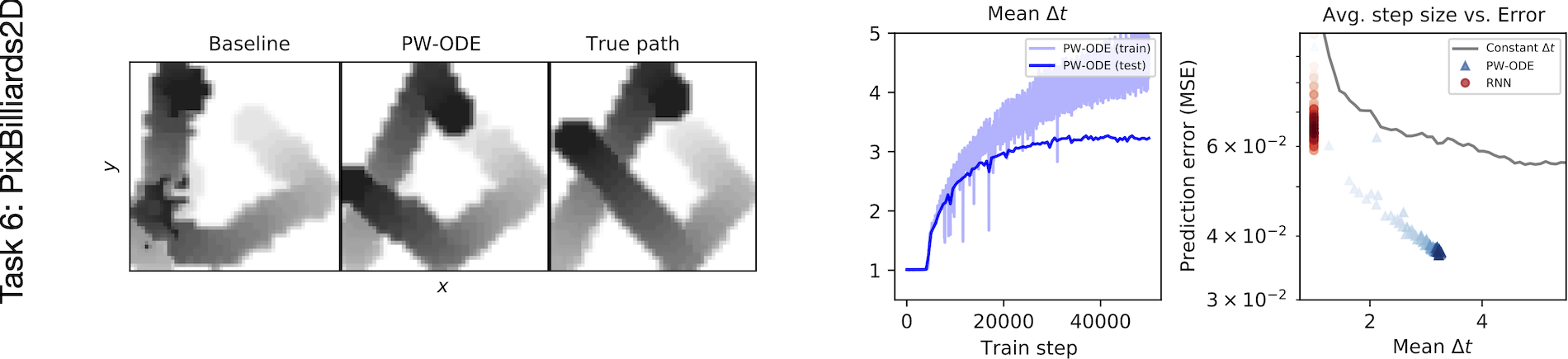
<img src="/assets/structural-optimization/mbb2.png" align="left" />
</pre>

<h2 id="optimizing-the-eves-of-a-gazebo-roof">Optimizing the eves of a gazebo roof</h2>
<p>Let’s turn to a slightly more challenging and interesting task. This is a design problem that came up recently at the engineering firm where I work. It consists of a gazebo roof that is 16’ wide and 4’ high (with a 2:1 pitch). The fixed points include the bottom region, where a large beam runs as well as a vertical center beam.</p>

<p>The dead load for the structure is 12-17 pounds per square foot (psf), the live load is 25 psf, snow load is 10 psf, wind load ranges from 10 psf downward to 4 psf upwards. Combining the vertical and horizontal forces with one another and estimating the worst-case net force on the roof, we obtain a vector with a magnitude that is 20 degrees (0.349 radians) off of the vertical. Putting all this together, we have a structural optimization problem which can be solved to obtain a support strucure for the roof.</p>

<div class="language-python highlighter-rouge"><div class="highlight"><pre class="highlight"><code><span class="k">def</span> <span class="nf">eves</span><span class="p">(</span><span class="n">width</span><span class="o">=</span><span class="mi">200</span><span class="p">,</span> <span class="n">height</span><span class="o">=</span><span class="mi">100</span><span class="p">,</span> <span class="n">density</span><span class="o">=</span><span class="mf">0.15</span><span class="p">,</span> <span class="n">theta</span><span class="o">=-</span><span class="mf">0.349</span><span class="p">):</span>
  <span class="c1"># theta is the angle (rad) between vertical and the net force on the roof
</span>  <span class="n">x_ix</span><span class="p">,</span> <span class="n">y_ix</span> <span class="o">=</span> <span class="mi">0</span><span class="p">,</span> <span class="mi">1</span>
  <span class="n">normals</span> <span class="o">=</span> <span class="n">np</span><span class="p">.</span><span class="n">zeros</span><span class="p">((</span><span class="n">width</span> <span class="o">+</span> <span class="mi">1</span><span class="p">,</span> <span class="n">height</span> <span class="o">+</span> <span class="mi">1</span><span class="p">,</span> <span class="mi">2</span><span class="p">))</span>
  <span class="n">normals</span><span class="p">[:,</span> <span class="o">-</span><span class="mi">1</span><span class="p">,</span> <span class="p">:]</span> <span class="o">=</span> <span class="mi">1</span>
  <span class="n">forces</span> <span class="o">=</span> <span class="n">np</span><span class="p">.</span><span class="n">zeros</span><span class="p">((</span><span class="n">width</span> <span class="o">+</span> <span class="mi">1</span><span class="p">,</span> <span class="n">height</span> <span class="o">+</span> <span class="mi">1</span><span class="p">,</span> <span class="mi">2</span><span class="p">))</span>
  <span class="n">start_coords</span><span class="p">,</span> <span class="n">stop_coords</span> <span class="o">=</span> <span class="p">(</span><span class="mi">0</span><span class="p">,</span> <span class="mi">0</span><span class="p">),</span> <span class="p">(</span><span class="n">width</span><span class="p">,</span> <span class="n">height</span><span class="p">)</span>

  <span class="kn">import</span> <span class="nn">skimage.draw</span>
  <span class="n">i</span><span class="p">,</span> <span class="n">j</span><span class="p">,</span> <span class="n">value</span> <span class="o">=</span> <span class="n">skimage</span><span class="p">.</span><span class="n">draw</span><span class="p">.</span><span class="n">line_aa</span><span class="p">(</span><span class="o">*</span><span class="n">start_coords</span><span class="p">,</span> <span class="o">*</span><span class="n">stop_coords</span><span class="p">)</span>
  <span class="n">forces</span><span class="p">[</span><span class="n">i</span><span class="p">,</span> <span class="n">j</span><span class="p">,</span> <span class="n">x_ix</span><span class="p">]</span> <span class="o">=</span> <span class="n">np</span><span class="p">.</span><span class="n">sin</span><span class="p">(</span><span class="n">theta</span><span class="p">)</span> <span class="o">*</span> <span class="n">np</span><span class="p">.</span><span class="n">minimum</span><span class="p">(</span><span class="n">forces</span><span class="p">[</span><span class="n">i</span><span class="p">,</span> <span class="n">j</span><span class="p">,</span> <span class="n">y_ix</span><span class="p">],</span> <span class="o">-</span><span class="n">value</span> <span class="o">/</span> <span class="n">width</span><span class="p">)</span>
  <span class="n">forces</span><span class="p">[</span><span class="n">i</span><span class="p">,</span> <span class="n">j</span><span class="p">,</span> <span class="n">y_ix</span><span class="p">]</span> <span class="o">=</span> <span class="n">np</span><span class="p">.</span><span class="n">cos</span><span class="p">(</span><span class="n">theta</span><span class="p">)</span> <span class="o">*</span> <span class="n">np</span><span class="p">.</span><span class="n">minimum</span><span class="p">(</span><span class="n">forces</span><span class="p">[</span><span class="n">i</span><span class="p">,</span> <span class="n">j</span><span class="p">,</span> <span class="n">y_ix</span><span class="p">],</span> <span class="o">-</span><span class="n">value</span> <span class="o">/</span> <span class="n">width</span><span class="p">)</span>
  <span class="k">return</span> <span class="n">normals</span><span class="p">,</span> <span class="n">forces</span><span class="p">,</span> <span class="n">density</span>

<span class="c1"># run the simulation and visualize the result
</span><span class="n">args</span> <span class="o">=</span> <span class="n">get_args</span><span class="p">(</span><span class="o">*</span><span class="n">eves</span><span class="p">())</span>
<span class="n">losses</span><span class="p">,</span> <span class="n">x</span><span class="p">,</span> <span class="n">frames</span> <span class="o">=</span> <span class="n">fast_stopt</span><span class="p">(</span><span class="n">args</span><span class="o">=</span><span class="n">args</span><span class="p">,</span> <span class="n">verbose</span><span class="o">=</span><span class="bp">True</span><span class="p">)</span>
</code></pre></div></div>
<pre class="outputarea">
Optimizing a problem with 66306 nodes
step 10, loss 1.01e+02, t=34.68s
step 20, loss 7.87e+00, t=69.54s
step 30, loss 3.05e+00, t=104.69s
step 40, loss 2.68e+00, t=138.80s
step 50, loss 2.53e+00, t=173.08s
step 60, loss 2.48e+00, t=206.53s
step 70, loss 2.47e+00, t=240.59s
step 80, loss 2.47e+00, t=278.73s
step 90, loss 2.46e+00, t=312.37s
step 100, loss 2.46e+00, t=347.35s
</pre>

<div class="imgcap" style="display: block; margin-left: auto; margin-right: auto; width:70%">
  <div style="width:100%; min-width:250px; display: inline-block; vertical-align: top;text-align:center;">
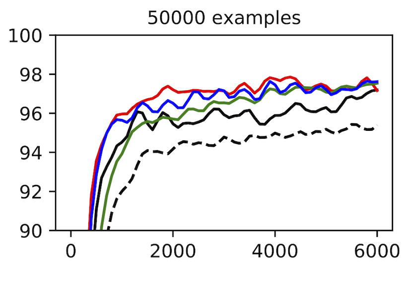
    <video id="eves_video" style="width:100%;min-width:250px;" poster="/assets/structural-optimization/eves.png">
      <source src="/assets/structural-optimization/eves.mp4" type="video/mp4" />
    </video>
    <button class="playbutton" id="eves_video_button" onclick="playPauseEves()">Play</button>
  </div>
</div>

<script> 
function playPauseEves() { 
  var video = document.getElementById("eves_video"); 
  var button = document.getElementById("eves_video_button");
  if (video.paused) {
    video.play();
    button.textContent = "Pause";}
  else {
    video.pause(); 
  button.textContent = "Play";}
} 
</script>

<h2 id="a-few-other-designs">A few other designs</h2>

<div class="language-python highlighter-rouge"><div class="highlight"><pre class="highlight"><code><span class="k">def</span> <span class="nf">causeway_bridge</span><span class="p">(</span><span class="n">width</span><span class="o">=</span><span class="mi">128</span><span class="p">,</span> <span class="n">height</span><span class="o">=</span><span class="mi">128</span><span class="p">,</span> <span class="n">density</span><span class="o">=</span><span class="mf">0.08</span><span class="p">,</span> <span class="n">deck_level</span><span class="o">=</span><span class="mf">0.2</span><span class="p">):</span>
  <span class="s">"""A bridge supported by columns at a regular interval."""</span>
  <span class="n">x_ix</span><span class="p">,</span> <span class="n">y_ix</span> <span class="o">=</span> <span class="mi">0</span><span class="p">,</span> <span class="mi">1</span>
  <span class="n">normals</span> <span class="o">=</span> <span class="n">np</span><span class="p">.</span><span class="n">zeros</span><span class="p">((</span><span class="n">width</span> <span class="o">+</span> <span class="mi">1</span><span class="p">,</span> <span class="n">height</span> <span class="o">+</span> <span class="mi">1</span><span class="p">,</span> <span class="mi">2</span><span class="p">))</span>
  <span class="n">normals</span><span class="p">[</span><span class="o">-</span><span class="mi">1</span><span class="p">,</span> <span class="o">-</span><span class="mi">1</span><span class="p">,</span> <span class="n">y_ix</span><span class="p">]</span> <span class="o">=</span> <span class="mi">1</span>
  <span class="n">normals</span><span class="p">[</span><span class="o">-</span><span class="mi">1</span><span class="p">,</span> <span class="p">:,</span> <span class="n">x_ix</span><span class="p">]</span> <span class="o">=</span> <span class="mi">1</span>
  <span class="n">normals</span><span class="p">[</span><span class="mi">0</span><span class="p">,</span> <span class="p">:,</span> <span class="n">x_ix</span><span class="p">]</span> <span class="o">=</span> <span class="mi">1</span>

  <span class="n">forces</span> <span class="o">=</span> <span class="n">np</span><span class="p">.</span><span class="n">zeros</span><span class="p">((</span><span class="n">width</span> <span class="o">+</span> <span class="mi">1</span><span class="p">,</span> <span class="n">height</span> <span class="o">+</span> <span class="mi">1</span><span class="p">,</span> <span class="mi">2</span><span class="p">))</span>
  <span class="n">forces</span><span class="p">[:,</span> <span class="nb">round</span><span class="p">(</span><span class="n">height</span> <span class="o">*</span> <span class="p">(</span><span class="mi">1</span> <span class="o">-</span> <span class="n">deck_level</span><span class="p">)),</span> <span class="n">y_ix</span><span class="p">]</span> <span class="o">=</span> <span class="o">-</span><span class="mi">1</span> <span class="o">/</span> <span class="n">width</span>
  <span class="k">return</span> <span class="n">normals</span><span class="p">,</span> <span class="n">forces</span><span class="p">,</span> <span class="n">density</span>

<span class="c1"># run the simulation and visualize the result
</span><span class="n">args</span> <span class="o">=</span> <span class="n">get_args</span><span class="p">(</span><span class="o">*</span><span class="n">causeway_bridge</span><span class="p">())</span>
<span class="n">args</span><span class="p">.</span><span class="n">opt_steps</span> <span class="o">=</span> <span class="mi">160</span> <span class="p">;</span> <span class="n">args</span><span class="p">.</span><span class="n">print_every</span> <span class="o">=</span> <span class="mi">20</span>
<span class="n">losses</span><span class="p">,</span> <span class="n">x</span><span class="p">,</span> <span class="n">frames</span> <span class="o">=</span> <span class="n">fast_stopt</span><span class="p">(</span><span class="n">args</span><span class="o">=</span><span class="n">args</span><span class="p">,</span> <span class="n">verbose</span><span class="o">=</span><span class="bp">True</span><span class="p">)</span>
</code></pre></div></div>
<pre class="outputarea">
Optimizing a problem with 33282 nodes
step 20, loss 6.45e+02, t=32.45s
step 40, loss 6.99e+01, t=66.31s
step 60, loss 6.22e+01, t=96.67s
step 80, loss 6.08e+01, t=127.47s
step 100, loss 6.01e+01, t=158.28s
step 120, loss 5.97e+01, t=188.59s
step 140, loss 5.90e+01, t=222.50s
step 160, loss 5.84e+01, t=253.61s
</pre>

<div class="imgcap" style="display: block; margin-left: auto; margin-right: auto; width:70%">
  <div style="width:100%; min-width:250px; display: inline-block; vertical-align: top;text-align:center;">
    <video id="causeway_video" style="width:100%;min-width:250px;" poster="/assets/structural-optimization/causeway.png">
      <source src="/assets/structural-optimization/causeway.mp4" type="video/mp4" />
    </video>
    <button class="playbutton" id="causeway_video_button" onclick="playPauseCauseway()">Play</button>
  </div>
</div>

<script> 
function playPauseCauseway() { 
  var video = document.getElementById("causeway_video"); 
  var button = document.getElementById("causeway_video_button");
  if (video.paused) {
    video.play();
    button.textContent = "Pause";}
  else {
    video.pause(); 
  button.textContent = "Play";}
} 
</script>

<div class="language-python highlighter-rouge"><div class="highlight"><pre class="highlight"><code><span class="k">def</span> <span class="nf">staggered_points</span><span class="p">(</span><span class="n">width</span><span class="o">=</span><span class="mi">64</span><span class="p">,</span> <span class="n">height</span><span class="o">=</span><span class="mi">256</span><span class="p">,</span> <span class="n">density</span><span class="o">=</span><span class="mf">0.3</span><span class="p">,</span> <span class="n">interval</span><span class="o">=</span><span class="mi">16</span><span class="p">,</span> <span class="n">break_symmetry</span><span class="o">=</span><span class="bp">False</span><span class="p">):</span>
  <span class="s">"""A staggered grid of points with downward forces, supported from below."""</span>
  <span class="n">x_ix</span><span class="p">,</span> <span class="n">y_ix</span> <span class="o">=</span> <span class="mi">0</span><span class="p">,</span> <span class="mi">1</span>
  <span class="n">normals</span> <span class="o">=</span> <span class="n">np</span><span class="p">.</span><span class="n">zeros</span><span class="p">((</span><span class="n">width</span> <span class="o">+</span> <span class="mi">1</span><span class="p">,</span> <span class="n">height</span> <span class="o">+</span> <span class="mi">1</span><span class="p">,</span> <span class="mi">2</span><span class="p">))</span>
  <span class="n">normals</span><span class="p">[:,</span> <span class="o">-</span><span class="mi">1</span><span class="p">,</span> <span class="n">y_ix</span><span class="p">]</span> <span class="o">=</span> <span class="mi">1</span>
  <span class="n">normals</span><span class="p">[</span><span class="mi">0</span><span class="p">,</span> <span class="p">:,</span> <span class="n">x_ix</span><span class="p">]</span> <span class="o">=</span> <span class="mi">1</span>
  <span class="n">normals</span><span class="p">[</span><span class="o">-</span><span class="mi">1</span><span class="p">,</span> <span class="p">:,</span> <span class="n">x_ix</span><span class="p">]</span> <span class="o">=</span> <span class="mi">1</span>

  <span class="n">forces</span> <span class="o">=</span> <span class="n">np</span><span class="p">.</span><span class="n">zeros</span><span class="p">((</span><span class="n">width</span> <span class="o">+</span> <span class="mi">1</span><span class="p">,</span> <span class="n">height</span> <span class="o">+</span> <span class="mi">1</span><span class="p">,</span> <span class="mi">2</span><span class="p">))</span>
  <span class="n">f</span> <span class="o">=</span> <span class="n">interval</span> <span class="o">**</span> <span class="mi">2</span> <span class="o">/</span> <span class="p">(</span><span class="n">width</span> <span class="o">*</span> <span class="n">height</span><span class="p">)</span>
  <span class="c1"># intentionally break horizontal symmetry?
</span>  <span class="n">forces</span><span class="p">[</span><span class="n">interval</span><span class="o">//</span><span class="mi">2</span><span class="o">+</span><span class="nb">int</span><span class="p">(</span><span class="n">break_symmetry</span><span class="p">)::</span><span class="n">interval</span><span class="p">,</span> <span class="p">::</span><span class="n">interval</span><span class="p">,</span> <span class="n">y_ix</span><span class="p">]</span> <span class="o">=</span> <span class="o">-</span><span class="n">f</span>
  <span class="n">forces</span><span class="p">[</span><span class="nb">int</span><span class="p">(</span><span class="n">break_symmetry</span><span class="p">)::</span><span class="n">interval</span><span class="p">,</span> <span class="n">interval</span><span class="o">//</span><span class="mi">2</span><span class="p">::</span><span class="n">interval</span><span class="p">,</span> <span class="n">y_ix</span><span class="p">]</span> <span class="o">=</span> <span class="o">-</span><span class="n">f</span>
  <span class="k">return</span> <span class="n">normals</span><span class="p">,</span> <span class="n">forces</span><span class="p">,</span> <span class="n">density</span>

<span class="c1"># run the simulation and visualize the result
</span><span class="n">args</span> <span class="o">=</span> <span class="n">get_args</span><span class="p">(</span><span class="o">*</span><span class="n">staggered_points</span><span class="p">())</span>
<span class="n">losses</span><span class="p">,</span> <span class="n">x</span><span class="p">,</span> <span class="n">frames</span> <span class="o">=</span> <span class="n">fast_stopt</span><span class="p">(</span><span class="n">args</span><span class="o">=</span><span class="n">args</span><span class="p">,</span> <span class="n">verbose</span><span class="o">=</span><span class="bp">True</span><span class="p">)</span>
</code></pre></div></div>
<pre class="outputarea">
Optimizing a problem with 33410 nodes
step 10, loss 1.91e+02, t=13.35s
step 20, loss 1.43e+02, t=26.34s
step 30, loss 6.96e+01, t=39.41s
step 40, loss 6.46e+01, t=52.50s
step 50, loss 4.44e+01, t=65.47s
step 60, loss 3.97e+01, t=78.36s
step 70, loss 3.76e+01, t=91.24s
step 80, loss 3.58e+01, t=104.05s
</pre>

<div class="imgcap" style="display: block; margin-left: auto; margin-right: auto; width:40%">
  <div style="width:100%; min-width:250px; display: inline-block; vertical-align: top;text-align:center;">
    <video id="points_video" style="width:100%;min-width:250px;" poster="/assets/structural-optimization/points.png">
      <source src="/assets/structural-optimization/points.mp4" type="video/mp4" />
    </video>
    <button class="playbutton" id="points_video_button" onclick="playPausePoints()">Play</button>
  </div>
</div>

<script> 
function playPausePoints() { 
  var video = document.getElementById("points_video"); 
  var button = document.getElementById("points_video_button");
  if (video.paused) {
    video.play();
    button.textContent = "Pause";}
  else {
    video.pause(); 
  button.textContent = "Play";}
} 
</script>

<div class="language-python highlighter-rouge"><div class="highlight"><pre class="highlight"><code><span class="k">def</span> <span class="nf">staircase</span><span class="p">(</span><span class="n">width</span><span class="o">=</span><span class="mi">256</span><span class="p">,</span> <span class="n">height</span><span class="o">=</span><span class="mi">256</span><span class="p">,</span> <span class="n">density</span><span class="o">=</span><span class="mf">0.15</span><span class="p">,</span> <span class="n">num_stories</span><span class="o">=</span><span class="mi">3</span><span class="p">):</span>
  <span class="s">"""A ramp that zig-zags upward, supported from the ground."""</span>
  <span class="n">x_ix</span><span class="p">,</span> <span class="n">y_ix</span> <span class="o">=</span> <span class="mi">0</span><span class="p">,</span> <span class="mi">1</span>
  <span class="n">normals</span> <span class="o">=</span> <span class="n">np</span><span class="p">.</span><span class="n">zeros</span><span class="p">((</span><span class="n">width</span> <span class="o">+</span> <span class="mi">1</span><span class="p">,</span> <span class="n">height</span> <span class="o">+</span> <span class="mi">1</span><span class="p">,</span> <span class="mi">2</span><span class="p">))</span>
  <span class="n">normals</span><span class="p">[:,</span> <span class="o">-</span><span class="mi">1</span><span class="p">,</span> <span class="p">:]</span> <span class="o">=</span> <span class="mi">1</span>

  <span class="kn">import</span> <span class="nn">skimage.draw</span>
  <span class="n">forces</span> <span class="o">=</span> <span class="n">np</span><span class="p">.</span><span class="n">zeros</span><span class="p">((</span><span class="n">width</span> <span class="o">+</span> <span class="mi">1</span><span class="p">,</span> <span class="n">height</span> <span class="o">+</span> <span class="mi">1</span><span class="p">,</span> <span class="mi">2</span><span class="p">))</span>
  <span class="k">for</span> <span class="n">story</span> <span class="ow">in</span> <span class="nb">range</span><span class="p">(</span><span class="n">num_stories</span><span class="p">):</span>
    <span class="n">parity</span> <span class="o">=</span> <span class="n">story</span> <span class="o">%</span> <span class="mi">2</span>
    <span class="n">start_coordinates</span> <span class="o">=</span> <span class="p">(</span><span class="mi">0</span><span class="p">,</span> <span class="p">(</span><span class="n">story</span> <span class="o">+</span> <span class="n">parity</span><span class="p">)</span> <span class="o">*</span> <span class="n">height</span> <span class="o">//</span> <span class="n">num_stories</span><span class="p">)</span>
    <span class="n">stop_coordiates</span> <span class="o">=</span> <span class="p">(</span><span class="n">width</span><span class="p">,</span> <span class="p">(</span><span class="n">story</span> <span class="o">+</span> <span class="mi">1</span> <span class="o">-</span> <span class="n">parity</span><span class="p">)</span> <span class="o">*</span> <span class="n">height</span> <span class="o">//</span> <span class="n">num_stories</span><span class="p">)</span>
    <span class="n">i</span><span class="p">,</span> <span class="n">j</span><span class="p">,</span> <span class="n">value</span> <span class="o">=</span> <span class="n">skimage</span><span class="p">.</span><span class="n">draw</span><span class="p">.</span><span class="n">line_aa</span><span class="p">(</span><span class="o">*</span><span class="n">start_coordinates</span><span class="p">,</span> <span class="o">*</span><span class="n">stop_coordiates</span><span class="p">)</span>
    <span class="n">forces</span><span class="p">[</span><span class="n">i</span><span class="p">,</span> <span class="n">j</span><span class="p">,</span> <span class="n">y_ix</span><span class="p">]</span> <span class="o">=</span> <span class="n">np</span><span class="p">.</span><span class="n">minimum</span><span class="p">(</span>
        <span class="n">forces</span><span class="p">[</span><span class="n">i</span><span class="p">,</span> <span class="n">j</span><span class="p">,</span> <span class="n">y_ix</span><span class="p">],</span> <span class="o">-</span><span class="n">value</span> <span class="o">/</span> <span class="p">(</span><span class="n">width</span> <span class="o">*</span> <span class="n">num_stories</span><span class="p">)</span>
    <span class="p">)</span>
  <span class="k">return</span> <span class="n">normals</span><span class="p">,</span> <span class="n">forces</span><span class="p">,</span> <span class="n">density</span>

<span class="c1"># run the simulation and visualize the result
</span><span class="n">args</span> <span class="o">=</span> <span class="n">get_args</span><span class="p">(</span><span class="o">*</span><span class="n">staircase</span><span class="p">())</span>
<span class="n">args</span><span class="p">.</span><span class="n">opt_steps</span> <span class="o">=</span> <span class="mi">100</span>
<span class="n">losses</span><span class="p">,</span> <span class="n">x</span><span class="p">,</span> <span class="n">frames</span> <span class="o">=</span> <span class="n">fast_stopt</span><span class="p">(</span><span class="n">args</span><span class="o">=</span><span class="n">args</span><span class="p">,</span> <span class="n">verbose</span><span class="o">=</span><span class="bp">True</span><span class="p">)</span>
</code></pre></div></div>
<pre class="outputarea">
Optimizing a problem with 132098 nodes
step 10, loss 9.65e+01, t=98.39s
step 20, loss 3.04e+01, t=197.26s
step 30, loss 7.37e+00, t=294.96s
step 40, loss 4.38e+00, t=390.48s
step 50, loss 3.98e+00, t=483.45s
step 60, loss 3.88e+00, t=575.68s
step 70, loss 3.86e+00, t=668.17s
step 80, loss 3.83e+00, t=758.19s
step 90, loss 3.82e+00, t=847.92s
step 100, loss 3.81e+00, t=939.67s
</pre>

<div class="imgcap" style="display: block; margin-left: auto; margin-right: auto; width:50%">
  <div style="width:100%; min-width:250px; display: inline-block; vertical-align: top;text-align:center;">
    <video id="staircase_video" style="width:100%;min-width:250px;" poster="/assets/structural-optimization/staircase.png">
      <source src="/assets/structural-optimization/staircase.mp4" type="video/mp4" />
    </video>
    <button class="playbutton" id="staircase_video_button" onclick="playPauseStaircase()">Play</button>
  </div>
</div>

<script> 
function playPauseStaircase() { 
  var video = document.getElementById("staircase_video"); 
  var button = document.getElementById("staircase_video_button");
  if (video.paused) {
    video.play();
    button.textContent = "Pause";}
  else {
    video.pause(); 
  button.textContent = "Play";}
} 
</script>

<div class="language-python highlighter-rouge"><div class="highlight"><pre class="highlight"><code><span class="k">def</span> <span class="nf">multistory_building</span><span class="p">(</span><span class="n">width</span><span class="o">=</span><span class="mi">128</span><span class="p">,</span> <span class="n">height</span><span class="o">=</span><span class="mi">512</span><span class="p">,</span> <span class="n">density</span><span class="o">=</span><span class="mf">0.2</span><span class="p">,</span> <span class="n">interval</span><span class="o">=</span><span class="mi">64</span><span class="p">):</span>
  <span class="n">x_ix</span><span class="p">,</span> <span class="n">y_ix</span> <span class="o">=</span> <span class="mi">0</span><span class="p">,</span> <span class="mi">1</span>
  <span class="n">normals</span> <span class="o">=</span> <span class="n">np</span><span class="p">.</span><span class="n">zeros</span><span class="p">((</span><span class="n">width</span> <span class="o">+</span> <span class="mi">1</span><span class="p">,</span> <span class="n">height</span> <span class="o">+</span> <span class="mi">1</span><span class="p">,</span> <span class="mi">2</span><span class="p">))</span>
  <span class="n">normals</span><span class="p">[:,</span> <span class="o">-</span><span class="mi">1</span><span class="p">,</span> <span class="n">y_ix</span><span class="p">]</span> <span class="o">=</span> <span class="mi">1</span>
  <span class="n">normals</span><span class="p">[</span><span class="o">-</span><span class="mi">1</span><span class="p">,</span> <span class="p">:,</span> <span class="n">x_ix</span><span class="p">]</span> <span class="o">=</span> <span class="mi">1</span>

  <span class="n">forces</span> <span class="o">=</span> <span class="n">np</span><span class="p">.</span><span class="n">zeros</span><span class="p">((</span><span class="n">width</span> <span class="o">+</span> <span class="mi">1</span><span class="p">,</span> <span class="n">height</span> <span class="o">+</span> <span class="mi">1</span><span class="p">,</span> <span class="mi">2</span><span class="p">))</span>
  <span class="n">forces</span><span class="p">[:,</span> <span class="p">::</span><span class="n">interval</span><span class="p">,</span> <span class="n">y_ix</span><span class="p">]</span> <span class="o">=</span> <span class="o">-</span><span class="mi">1</span> <span class="o">/</span> <span class="n">width</span>
  <span class="k">return</span> <span class="n">normals</span><span class="p">,</span> <span class="n">forces</span><span class="p">,</span> <span class="n">density</span>

<span class="c1"># run the simulation and visualize the result
</span><span class="n">args</span> <span class="o">=</span> <span class="n">get_args</span><span class="p">(</span><span class="o">*</span><span class="n">multistory_building</span><span class="p">())</span>
<span class="n">args</span><span class="p">.</span><span class="n">opt_steps</span> <span class="o">=</span> <span class="mi">160</span> <span class="p">;</span> <span class="n">args</span><span class="p">.</span><span class="n">print_every</span> <span class="o">=</span> <span class="mi">10</span>
<span class="n">losses</span><span class="p">,</span> <span class="n">x</span><span class="p">,</span> <span class="n">frames</span> <span class="o">=</span> <span class="n">fast_stopt</span><span class="p">(</span><span class="n">args</span><span class="o">=</span><span class="n">args</span><span class="p">,</span> <span class="n">verbose</span><span class="o">=</span><span class="bp">True</span><span class="p">)</span>
</code></pre></div></div>
<pre class="outputarea">
Optimizing a problem with 132354 nodes
step 10, loss 1.28e+04, t=72.03s
step 20, loss 8.77e+03, t=144.31s
step 30, loss 7.23e+03, t=215.94s
step 40, loss 1.74e+03, t=289.13s
step 50, loss 9.65e+02, t=362.98s
step 60, loss 8.40e+02, t=434.95s
step 70, loss 8.06e+02, t=506.56s
step 80, loss 7.97e+02, t=577.98s
step 90, loss 7.89e+02, t=648.11s
step 100, loss 7.87e+02, t=718.23s
step 110, loss 7.85e+02, t=787.93s
step 120, loss 7.83e+02, t=857.21s
step 130, loss 7.82e+02, t=927.52s
step 140, loss 7.81e+02, t=996.80s
step 150, loss 7.79e+02, t=1066.46s
step 160, loss 7.77e+02, t=1135.57s
</pre>
<div class="imgcap" style="display: block; margin-left: auto; margin-right: auto; width:80%">
  <div style="width:100%; min-width:250px; display: inline-block; vertical-align: top;text-align:center;">
    <video id="building_video" style="width:100%;min-width:250px;" poster="/assets/structural-optimization/building.png">
      <source src="/assets/structural-optimization/building.mp4" type="video/mp4" />
    </video>
    <button class="playbutton" id="building_video_button" onclick="playPauseBuilding()">Play</button>
  </div>
</div>

<script> 
function playPauseBuilding() { 
  var video = document.getElementById("building_video"); 
  var button = document.getElementById("building_video_button");
  if (video.paused) {
    video.play();
    button.textContent = "Pause";}
  else {
    video.pause(); 
  button.textContent = "Play";}
} 
</script>

<p>There are many, many more structures in <a href="https://arxiv.org/src/1909.04240v2/anc/all-designs.pdf">this supplement</a> from <a href="https://scholar.google.com/scholar?hl=en&amp;as_sdt=0%2C38&amp;q=Neural+reparameterization+improves+structural+optimization&amp;btnG=">Hoyer et al. 2019</a>. The problem setups are all listed <a href="https://github.com/google-research/neural-structural-optimization/blob/1c11b8c6ef50274802a84cf1a244735c3ed9394d/neural_structural_optimization/problems.py">here</a>.</p>

<h2 id="discussion">Discussion</h2>

<p>In sci-fi representations of the healthy cities of the future, we often find manmade structures that are well integrated with their natural surroundings. Sometimes we even see a convergence where nature has adapted to the city and the city has adapted to nature. The more decadent cities, on the other hand, tend to define themselves in opposition to the patterns of nature. Their architecture is more blocky and inorganic. Perhaps tools like structural optimization can help us build the healthy cities of the future – and steer clear of the decadent ones.</p>

<div class="imgcap_noborder" style="display: block; margin-left: auto; margin-right: auto; width:100%; min-width:320px;">
  <img src="/assets/structural-optimization/asgard.jpeg" />
  <div style="text-align:center; display:block; margin-left: auto; margin-right: auto; width:100%">The city of Asgard from <i>Thor</i></div>
</div>

<h2 id="footnotes">Footnotes</h2>

<script>
    function getBrowserSize(){
       var w, h;

         if(typeof window.innerWidth != 'undefined')
         {
          w = window.innerWidth; //other browsers
          h = window.innerHeight;
         } 
         else if(typeof document.documentElement != 'undefined' && typeof      document.documentElement.clientWidth != 'undefined' && document.documentElement.clientWidth != 0) 
         {
          w =  document.documentElement.clientWidth; //IE
          h = document.documentElement.clientHeight;
         }
         else{
          w = document.body.clientWidth; //IE
          h = document.body.clientHeight;
         }
       return {'width':w, 'height': h};
}

if(parseInt(getBrowserSize().width) < 800){
 document.getElementById("longEqnWithLargeScript_A").style.display = "none";
}
if(parseInt(getBrowserSize().width) > 800){
 document.getElementById("longEqnWithSmallScript_A").style.display = "none";
}

if(parseInt(getBrowserSize().width) < 800){
 document.getElementById("longEqnWithLargeScript_B").style.display = "none";
}
if(parseInt(getBrowserSize().width) > 800){
 document.getElementById("longEqnWithSmallScript_B").style.display = "none";
}
</script>

<div class="footnotes" role="doc-endnotes">
  <ol>
    <li id="fn:fn1" role="doc-endnote">
      <p><a href="https://www.topopt.mek.dtu.dk/-/media/subsites/topopt/apps/dokumenter-og-filer-til-apps/topopt88.pdf?la=da&amp;hash=E80FAB2808804A29FFB181CA05D2EEFECAA86686">Andreassen et al (2010)</a> use a cone filter; we found that a Gaussian filter gave similar results and was easier to implement. <a href="#fnref:fn1" class="reversefootnote" role="doc-backlink">&#8617;</a></p>
    </li>
    <li id="fn:fn2" role="doc-endnote">
      <p>Deriving the specific entries of the element stiffness matrix takes quite a few steps. We won’t go through all of them here, but you can walk yourself through them using <a href="http://solidmechanics.org/text/Chapter7_2/Chapter7_2.htm">this textbook chapter</a>. <a href="#fnref:fn2" class="reversefootnote" role="doc-backlink">&#8617;</a></p>
    </li>
  </ol>
</div>]]></content><author><name>Sam Greydanus</name></author><summary type="html"><![CDATA[Structural optimization lets us design trusses, bridges, and buildings starting from the physics of elastic materials. Let's code it up, from scratch, in 180 lines.]]></summary></entry><entry><title type="html">How Simulating the Universe Could Yield Quantum Mechanics</title><link href="http://greydanus.github.io/2022/03/27/how-simulating/" rel="alternate" type="text/html" title="How Simulating the Universe Could Yield Quantum Mechanics" /><published>2022-03-27T11:00:00+00:00</published><updated>2022-03-27T11:00:00+00:00</updated><id>http://greydanus.github.io/2022/03/27/how-simulating</id><content type="html" xml:base="http://greydanus.github.io/2022/03/27/how-simulating/"><![CDATA[<!-- ## The Universe as a Simulation -->

<div class="imgcap_noborder" style="display: block; margin-left: auto; margin-right: auto; width:15%; min-width:200px;">
  <img src="/assets/how-simulating/galaxy.png" />
</div>

<p>Let’s imagine the universe is being simulated. Based on what we know about physics, what can we say about how the simulation would be implemented? Well, it would probably have:</p>

<ol>
  <li><strong>Massive parallelism.</strong> Taking advantage of the fact that, in physics, all interactions are local and limited by the speed of light, one could parallelize the simulation. Spatially adjacent regions would run on the same CPUs whereas spatially distant regions would run on separate CPUs.<sup id="fnref:fn1" role="doc-noteref"><a href="#fn:fn1" class="footnote" rel="footnote">1</a></sup></li>
  <li><strong>Conservation laws enforced.</strong> Physics is built on the idea that certain quantities are strictly conserved. Scalar quantities like <a href="https://en.wikipedia.org/wiki/Conservation_law#Exact_laws">mass-energy</a> are conserved, as are vector quantities like <a href="https://en.wikipedia.org/wiki/Conservation_law#Exact_laws">angular momentum</a>.<sup id="fnref:fn2" role="doc-noteref"><a href="#fn:fn2" class="footnote" rel="footnote">2</a></sup></li>
  <li><strong>Binary logic.</strong> Our computers use discrete, binary logic to represent and manipulate information. Non-discrete numbers are represented with sequences of discrete symbols (see <a href="https://en.wikipedia.org/wiki/Single-precision_floating-point_format">float32</a>). Let’s assume our simulation does the same thing.</li>
  <li><strong>Adaptive computation.</strong> To simulate the universe efficiently, we would want to spend most of our compute time on regions where a lot of matter and energy are concentrated: that’s where the dynamics would be most complex. So we’d probably want to use a <a href="https://en.wikipedia.org/wiki/Lagrangian_particle_tracking">particle-based (Lagrangian) simulation</a> of some sort.</li>
  <li><strong>Isotropy.</strong> Space would be <a href="https://en.wikipedia.org/wiki/Isotropy">uniform in all directions</a>; physics would be invariant under rotation.</li>
</ol>

<p>We can determine whether these are reasonable assumptions by checking that they hold true for existing state-of-the-art physics simulations. It turns out that they hold true for the best <a href="https://www.myroms.org/">oceanography</a>, <a href="https://confluence.ecmwf.int/display/S2S/ECMWF+model+description">meteorology</a>, <a href="https://arxiv.org/abs/0810.5757">plasma</a>, <a href="https://en.wikipedia.org/wiki/NEMO_(Stellar_Dynamics_Toolbox)">cosmology</a>, and <a href="https://en.wikipedia.org/wiki/Computational_fluid_dynamics">computational fluid dynamics</a> models. So, having laid out some basic assumptions about how our simulation would be implemented, let’s look at their implications.</p>

<h2 id="enforcing-conservation-laws-in-parallel">Enforcing conservation laws in parallel</h2>

<p>The first thing to see is that assumptions 1 and 2 are in tension with one another. In order to ensure that a quantity (eg mass-energy) is conserved, you need to sum that quantity across the entire simulation, determine whether a correction is needed, and then apply that correction to the system as a whole. Computationally, this requires a synchronous <a href="https://en.wikipedia.org/wiki/Reduction_operator">reduction operation</a> and an element-wise divide at virtually every timestep.</p>

<div class="imgcap_noborder" style="display: block; margin-left: auto; margin-right: auto; width:100%">
  <img src="/assets/how-simulating/fig1.png" />
      <div class="thecap" style="text-align:left; display:block; margin-left: auto; margin-right: auto; width:100%">
  A conceptual outline of a large-scale physics simulation where different regions of space are being simulated in parallel. This parallelization is possible because nothing can travel faster than the speed of light; thus the separate regions can be simulated independently over short timescales.
  </div>
</div>

<p>When you write a single-threaded physics simulation, this can account for about half of the computational cost (these <a href="https://github.com/greydanus/optimize_wing/blob/3d661cae6ca6a320981fd5fc29848e1233d891cd/simulate.py#L57">fluid</a> and <a href="https://github.com/google-research/neural-structural-optimization/blob/1c11b8c6ef50274802a84cf1a244735c3ed9394d/neural_structural_optimization/topo_physics.py#L236">topology</a> simulations are good examples). As you parallelize your simulation more and more, you can expect the cost of enforcing conservation laws to grow higher in proportion. This is because simulating dynamics is pretty easy to do in parallel. But enforcing system-wide conservation laws requires transferring data between distant CPU cores and keeping them more or less in sync. As a result, enforcing conservation laws in this manner quickly grows to be a limiting factor on runtime. We find ourselves asking: <em>is there a more parallelizable approach to enforcing global conservation laws?</em></p>

<p>One option is to use a <a href="https://en.wikipedia.org/wiki/Finite_volume_method">finite volume method</a> to keep track of quantities moving between grid cells rather than absolute values. If we don’t care about <em>exactly</em> enforcing a conservation law, then this may be sufficient. We should note, though, that under a finite volume scheme small rounding and integration errors will occur and over time they will cause the globally-conserved quantity to change slightly. (More speculatively, this may be a particularly serious problem if people in the simulation are liable to stumble upon this phenomenon and exploit it adversarially to create or destroy energy.)</p>

<p>If we want to <em>strictly</em> enforce a globally-conserved quantity in a fully parallel manner, there is a third option that we could try: we could quantize it. We could quantize energy, for example, and then only transfer it in the form of discrete packets.</p>

<p>To see why this would be a good idea, let’s use financial markets as an analogy. Financial markets are massively parallel and keeping a proper accounting of the total amount of currency in circulation is very important. So they allow currency to function as a continuous quantity on a practical level, but they quantize it at a certain scale by making small measures of value (pennies) indivisible. We could enforce conservation of energy in the same way, for the same reasons.</p>

<h2 id="conserving-vector-quantities">Conserving vector quantities</h2>

<p>Quantization may work well for conserving scalar values like energy. But what about conserving vector quantities like angular momentum? In these cases, isotropy/rotational symmetry (assumption 5) makes things difficult. Isotropy says that our simulation will be invariant under rotation, but if we quantized the directions of our angular momentum vectors, we would be unable to represent all spatial directions equally. We’d get <a href="https://en.wikipedia.org/wiki/Round-off_error">rounding errors</a> which would compound over time.</p>

<p>So how are we to implement exact conservation of vector quantities? One option is to require that one particle’s vector quantities always be defined in reference to some other particle’s vector quantities. This could be implemented by creating multiple <a href="https://en.wikipedia.org/wiki/Pointer_(computer_programming)">pointer references</a> to a single variable and then giving each of those pointers to a different particle. As a concrete example, we might imagine an atom releasing energy in the form of two photons. The polarization angle of the first photon could be expressed as a 90\(^\circ\) clockwise rotation of a pointer to variable <code class="language-plaintext highlighter-rouge">x</code>. Meanwhile, the polarization angle of the second photon could be expressed as a 90\(^\circ\) counterclockwise rotation of a pointer to the same variable <code class="language-plaintext highlighter-rouge">x</code>. As we advance our simulation through time, the polarization angles of the two photons would change. Perhaps some small integration and rounding errors would accumulate. But even if that happens, we can say with confidence that the relative difference in polarization angle will be a constant 180\(^\circ\). In this way, we could enforce conservation of angular momentum in parallel across the entire simulation.</p>

<p>We should recognize that this approach comes at a price. It demands that we sacrifice <em>locality</em>, the principle that an object is influenced directly only by its immediate surroundings. It’s one of the most sacred principles in physics. This gets violated in the example of the two photons because a change in the polarization of the first photon will update the value of <code class="language-plaintext highlighter-rouge">x</code>, implicitly changing the polarization of the second photon.</p>

<div class="imgcap_noborder" style="display: block; margin-left: auto; margin-right: auto; width:100%">
  <img src="/assets/how-simulating/fig2.png" />
    <div class="thecap" style="text-align:left; display:block; margin-left: auto; margin-right: auto; width:100%">
  This figure is inspired by the experimental setup of <a href="https://drive.google.com/file/d/1ac4E87cKMgp90PfoNeTaRiVE3HEC9ubJ/view?usp=sharing">Clauser and Horne (1974)</a> used to test the Bell inequality. Here we are hypothesizing the existence of a shared hidden variable <i>x</i> which, when updated due to the left photon's interaction with a polarizer, also affects the right photon's polarization.
  </div>
</div>

<p>Interestingly, the mechanics of this nonlocal relationship would predict a violation of <a href="https://www.youtube.com/watch?v=zcqZHYo7ONs&amp;vl=en">Bell’s inequality</a> which would match experimental results. Physicists agree that violation of Bell’s inequality implies that nature violates either <em>realism</em>, the principle that reality exists with definite properties even when not being observed, or locality. Since locality is seen as a more fundamental principle than realism, the modern consensus is that quantum mechanics violates realism. In this line of thinking, entangled particles cannot be said to have deterministic states and instead exist in a state of superposition until they are measured. But in our simulated universe, realism would be preserved and locality would be sacrificed. Entangled particles would have definite states but sometimes those states would change due to shared references to spatially distant “twins.”<sup id="fnref:fn4" role="doc-noteref"><a href="#fn:fn4" class="footnote" rel="footnote">3</a></sup> To see how this would work in practice, try simulating it yourself at the link below.</p>

<div style="display: block; margin-left: auto; margin-right:auto; width:100%; text-align:center;">
  <a href="https://colab.research.google.com/drive/1b_DJo27Cq9E6zxSD9KpvyilaVV512SkU?usp=sharing" id="linkbutton" target="_blank"><span class="colab-span">Run</span> in browser</a>
</div>

<h2 id="explaining-the-double-slit-experiment">Explaining the double slit experiment</h2>

<p>Our findings thusfar may lead us to ask whether other quantum mechanical phenomena can be derived from the simulation <em>ansatz</em>. For example, what could be causing the wave-particle duality of light as seen in the double slit experiment?</p>

<p>The important idea here is <a href="https://en.wikipedia.org/wiki/Filter_(large_eddy_simulation)">filtering</a>. Filtering is a common technique where a Gaussian or cone filter is convolved with a grid in order to smooth out the physics and eliminate grid-level pathologies. This step is essential – for example, these <a href="https://github.com/greydanus/optimize_wing/blob/3d661cae6ca6a320981fd5fc29848e1233d891cd/simulate.py#L83">fluid</a> and <a href="https://github.com/google-research/neural-structural-optimization/blob/1c11b8c6ef50274802a84cf1a244735c3ed9394d/neural_structural_optimization/topo_physics.py#L84">topology</a> simulations would not work without it.</p>

<p>How would one implement filtering in a large-scale, particle-based simulation of the universe? Well, if the simulation were particle-based instead of grid-based, we couldn’t apply a Gaussian or cone filter. An alternative would be to simulate the dynamics of each particle using ensembles of virtual particles. One could initialize a group of these virtual particles with slightly different initial conditions and then simulate all of them through time. If you allowed these virtual particles to interact with other virtual particles in the ensemble, the entire ensemble would collectively behave as though it were a wave.</p>

<div class="imgcap_noborder" style="display: block; margin-left: auto; margin-right: auto; width:100%">
  <img src="/assets/how-simulating/fig3.png" style="width:90%" />
    <div class="thecap" style="text-align:left; display:block; margin-left: auto; margin-right: auto; width:100%">
  Wave-particle behavior of a photon as a consequence of using an ensemble of virtual particles and selecting just one to transfer a quanta of energy to the photoreceptor.
  </div>
</div>

<p>You might notice that there is a tension between this spatially delocalized, wave-like behavior (a consequence of filtering, which is related to assumption 3) and the conservation/quantization of quantities like energy (assumption 2). The tension is this: when a wave interacts with an object, it transfers energy in a manner that is delocalized and proportionate to its amplitude at a given location. But we have decided to quantize energy in order to keep an exact accounting of it across our simulation. So when our ensemble of particles interacts with some matter, it must transfer exactly one quanta of energy and it must do so at one particular location.</p>

<p>The simplest way to implement this would be to choose one particle out of the ensemble and allow it to interact with other matter and transfer energy. The rest of the particles in the ensemble would be removed from the simulation upon coming into contact with other matter. The interesting thing about this approach is that it could help explain the wave-particle duality of subatomic particles such as photons. For example, it could be used to reproduce the empirical results of the double slit experiment in a fully deterministic manner.<sup id="fnref:fn6" role="doc-noteref"><a href="#fn:fn6" class="footnote" rel="footnote">4</a></sup></p>

<h2 id="but-classical-computers-cant-simulate-quantum-effects">“But classical computers can’t simulate quantum effects”</h2>

<p>It is generally accepted that the cost of simulating \(N\) entangled particles, each with \(d\) degrees of freedom, grows as \(d^{N}\). This means that simulating a quantum system with a classical computer becomes prohibitively expensive for even small groups of particles. And if you simulate such systems probabilistically, you will inevitably encounter cases where the simulated physics doesn’t match reality.<sup id="fnref:fn5" role="doc-noteref"><a href="#fn:fn5" class="footnote" rel="footnote">5</a></sup> If it’s that difficult for classical computers to simulate quantum effects – and the universe is quantum mechanical – then isn’t this entire thought experiment destined to fail?</p>

<p>Perhaps not. Claims about the difficulty of simulating quantum effects are based on <a href="https://en.wikipedia.org/wiki/Quantum_indeterminacy">quantum indeterminacy</a>, the idea that entangled particles do not have definite states prior to measurement. This interpretation of quantum effects comes about when we sacrifice the assumption of realism. But if we sacrifice locality (as we have done in this article), then we need not sacrifice realism. In a world where entangled particles can affect each other’s states instantaneously at a distance (nonlocality), they can always have specific states (realism) and still produce the empirical behaviors (<a href="https://en.wikipedia.org/wiki/Bell%27s_theorem#Experiments">violation of Bell’s theorem</a>) that consitute the basis of the theory of quantum mechanics. This sort of world could be simulated on a classical computer.</p>

<h2 id="testing-our-hypothesis">Testing our hypothesis</h2>

<p>Suppose the ideas we have discussed are an accurate model of reality. How would we test them? We could start by showing that in quantum mechanics, realism is actually preserved whereas locality is not. To that end, here’s one potential experiment:</p>

<p><em>We set up the apparatus used to test Bell’s inequality. Entangled photons emerge from a source and head in opposite directions. Eventually they get their polarizations measured. We allow the first photon in the pair to enter a double slit experiment. As it passes through the double slit, it interferes with itself, producing a wavelike diffraction pattern on the detector.</em></p>

<div class="imgcap_noborder" style="display: block; margin-left: auto; margin-right: auto; width:100%">
  <img src="/assets/how-simulating/fig4.png" style="width:80%" />
  <div class="thecap" style="text-align:left; display:block; margin-left: auto; margin-right: auto; width:100%">
  One possible means of testing the hypothesis we have outlined. If photons used to test the Bell inequality behave in this manner when they encounter a double slit setup, one could use them to transmit information faster than the speed of light, violating the locality assumption.
  </div>
</div>

<p><em>Then we change the experiment by measuring the second photon in the pair before the first photon reaches the double slit. This will break the entanglement, causing both photons to enter well-defined polarization states. When this happens, the first photon will behave like a particle as it passes through the double slit experiment. This would be a surprising result because such a setup would violate the locality assumption<sup id="fnref:fn3" role="doc-noteref"><a href="#fn:fn3" class="footnote" rel="footnote">6</a></sup> and could be used to transmit information faster than light.</em></p>

<h2 id="closing-thoughts">Closing thoughts</h2>

<p>To the followers of Plato, the world of the senses was akin to shadows dancing on the wall of a cave. The essential truths and realities of life were not to be found on the wall at all, but rather somewhere else in the cave in the form of real dancers and real flames. A meaningful life was to be spent seeking to understand those forms, elusive though they might be.</p>

<p>In this post, we took part in that tradition by using our knowledge of physics simulations to propose a new interpretation of quantum mechanics. It’s hard to know whether we do indeed live in a simulation. Perhaps we will never know. But at the very least, the idea serves as a good basis for a thought-provoking discussion.</p>

<h2 id="footnotes">Footnotes</h2>

<script language="javascript">
function hideShowNote() {
  var x = document.getElementById("note_to_reader");
  var y = document.getElementById("note_toggle");
  if (x.style.display === "none") {
    x.style.display = "inline"; y.textContent = "(–)"
  } else {
    x.style.display = "none"; y.textContent = "(+)"
  }
}
</script>

<div class="footnotes" role="doc-endnotes">
  <ol>
    <li id="fn:fn1" role="doc-endnote">
      <p>This is connected to the notion of <a href="https://plato.stanford.edu/entries/cellular-automata/#CAModeReal">cellular automata as models of reality</a>. <a href="#fnref:fn1" class="reversefootnote" role="doc-backlink">&#8617;</a></p>
    </li>
    <li id="fn:fn2" role="doc-endnote">
      <p>As a subset of conservation of angular momentum, <a href="https://www.nature.com/articles/s41467-019-10939-x">polarization</a> is also conserved. This is relevant to later examples which assume conservation of polarization. <a href="#fnref:fn2" class="reversefootnote" role="doc-backlink">&#8617;</a></p>
    </li>
    <li id="fn:fn4" role="doc-endnote">
      <p>Physicists have certainly entertained the idea of using non-local theories to explain Bell’s inequality. One of the reasons these theories are not more popular is that <a href="https://drive.google.com/file/d/1RTlV08KhQ7lNwOukbNcMok0f6E42uMyI/view?usp=sharing">Groblacher et al, 2007</a> and others have reported experimental results that rule out some of the more reasonable options (eg Leggett-style non-local theories). But the idea we are proposing here is somewhat more radical; it would permit information to travel faster than the speed of light, violating the <a href="https://en.wikipedia.org/wiki/No-communication_theorem">No-communication theorem</a>. Of course, the only information that could be communicated faster than the speed of light would be <em>whether a given pair of particles is in a superposition of states or not</em>. Look at the “Testing our hypothesis” section for more discussion on this topic. <a href="#fnref:fn4" class="reversefootnote" role="doc-backlink">&#8617;</a></p>
    </li>
    <li id="fn:fn6" role="doc-endnote">
      <p>Update (May 16, 2022): I tried to <a href="https://colab.research.google.com/drive/1Ayh4mGyx4Td63nfF2-bLd5cQJaGQLEz5?usp=sharing">code this up</a> and encountered some problems. First of all, it’s a nontrivial simulation problem. But apart from that, it’s difficult to achieve wavelike behaviors across the group without faster-than-light propagation of electric fields (which I suspect is nonphysical). I suspect that this filtering path is still a viable route to explaining the double slit experiment, but I now believe that the implementation details may look a bit different. One idea Jason Yosinski suggested was: what if our simulator was solving a PDE in both the spatial domain <em>and</em> the frequency domain and occasionally, whenever a spatial pattern got too diffuse, it would be transferred over to the frequency domain. Conversely, whenever a frequency pattern got too localized, it would be transferred over to the spatial domain. This could help to explain, for example <a href="https://en.wikipedia.org/wiki/Vacuum_energy">particle generation in a vacuum</a>. More on this in the future. <a href="#fnref:fn6" class="reversefootnote" role="doc-backlink">&#8617;</a></p>
    </li>
    <li id="fn:fn5" role="doc-endnote">
      <p>See Section 5 of Feynman’s “<a href="https://www.taylorfrancis.com/chapters/edit/10.1201/9780429500459-11/simulating-physics-computers-richard-feynman">Simulating physics with computers</a>” <a href="#fnref:fn5" class="reversefootnote" role="doc-backlink">&#8617;</a></p>
    </li>
    <li id="fn:fn3" role="doc-endnote">
      <p>Relatedly, it will also violate the <a href="https://en.wikipedia.org/wiki/No-communication_theorem">no-communication theorem</a>, which is a core claim of quantum mechanics. <a href="#fnref:fn3" class="reversefootnote" role="doc-backlink">&#8617;</a></p>
    </li>
  </ol>
</div>]]></content><author><name>Sam Greydanus</name></author><summary type="html"><![CDATA[We look at the logistics of simulating the universe. We find that enforcing conservation laws, isotropy, etc. in parallel could lead to quantum-like effects.]]></summary></entry><entry><title type="html">Dissipative Hamiltonian Neural Networks</title><link href="http://greydanus.github.io/2022/01/25/dissipative-hnns/" rel="alternate" type="text/html" title="Dissipative Hamiltonian Neural Networks" /><published>2022-01-25T11:00:00+00:00</published><updated>2022-01-25T11:00:00+00:00</updated><id>http://greydanus.github.io/2022/01/25/dissipative-hnns</id><content type="html" xml:base="http://greydanus.github.io/2022/01/25/dissipative-hnns/"><![CDATA[<div class="imgcap_noborder" style="display: block; margin-left: auto; margin-right: auto; width:100%">
  <img src="/assets/dissipative-hnns/hero.jpg" />
  <div class="thecap" style="text-align:left; display:block; margin-left: auto; margin-right: auto; width:100%">
  Dissipative HNNs (D-HNNs) improve upon <a href="https://greydanus.github.io/2019/05/15/hamiltonian-nns/">Hamiltonian Neural Networks</a>. They output two scalar functions, denoted here by <i><b>H</b></i> and <i><b>D</b></i>. The first of these two, <i><b>H</b></i>, is the Hamiltonian. We use its symplectic gradient to model energy-conserving dynamics. The second, <i><b>D</b></i>, is the Rayleigh dissipation function. We use it to model the dissipative component of the system. The addition of this dissipation function allows D-HNNs to model systems where energy is not quite conserved, as, for example, in the case of the damped mass-spring system shown here.
  </div>
</div>

<div style="display: block; margin-left: auto; margin-right:auto; width:100%; text-align:center;">
  <a href="https://arxiv.org/abs/2201.10085" id="linkbutton" target="_blank">Read the paper</a>
  <a href="https://github.com/DrewSosa/dissipative_hnns" id="linkbutton" target="_blank">Get the code</a>
</div>

<h2 id="a-sea-of-change">A sea of change</h2>

<p>We are immersed in a complex, dynamic world where change is the only constant. And yet there are certain patterns to this change that suggest natural laws. These laws include conservation of mass, energy, and momentum. Taken together, they constitute a powerful simplifying constraint on reality. Indeed, physics tells us that a small set of laws and their associated invariances are at the heart of all natural phenomena. Whether we are studying weather, ocean currents, earthquakes, or molecular interactions, we should take care to respect these laws. And when we apply learning algorithms to these domains, we should ensure that they, too, respect these laws.</p>

<p>We can do this by building models that are primed to learn invariant quantities from data: these models include <a href="https://greydanus.github.io/2019/05/15/hamiltonian-nns/">HNNs</a>, <a href="https://greydanus.github.io/2020/03/10/lagrangian-nns/">LNNs</a>, and a <a href="https://scholar.google.com/scholar?hl=en&amp;as_sdt=0%2C38&amp;q=hamiltonian+neural+networks&amp;btnG=">growing class</a> of <a href="https://scholar.google.com/scholar?hl=en&amp;as_sdt=0,38&amp;q=symplectic+neural+networks">related models</a>. But one problem with these models is that, for the most part, they can only handle data where some quantity (such as energy) is exactly conserved. If the data is collected in the real world and there is even a small amount of friction, then these models struggle. In this post, we introduce Dissipative HNNs, a class of models which can learn conservation laws from data even when energy isn’t perfectly conserved.</p>

<div class="imgcap_noborder" style="display: block; margin-left: auto; margin-right: auto; width:100%">
  <img src="/assets/dissipative-hnns/sea_of_change.jpg" />
  <div class="thecap" style="text-align:left; display:block; margin-left: auto; margin-right: auto; width:100%">
  We live in a sea of change. But no matter how complex a system's dynamics are, they can always be decomposed into the sum of dissipative dynamics and conservative dynamics.
  </div>
</div>

<p>The core idea is to use a neural network to parameterize both a Hamiltonian <em>and</em> a Rayleigh dissipation function. During training, the Hamiltonian function fits the conservative (rotational) component of the dynamics whereas the Rayleigh function fits the dissipative (irrotational) component. Let’s dive in to how this works.</p>

<h2 id="a-quick-theory-section">A quick theory section</h2>

<p><strong>The Hamiltonian function.</strong> The Hamiltonian \(\mathcal{H}(\textbf{q},\textbf{p})\) is scalar function where by definition \( \frac{\partial \mathcal{H}}{\partial \textbf{p}} = \frac{\partial \textbf{q}}{dt},  -\frac{\partial \mathcal{H}}{\partial \textbf{q}} = \frac{\partial \textbf{p}}{dt} \). This constraint tells us that, even as the position and momentum coordinates of the system \(\textbf{(q, p)}\) change, the scalar output \(\mathcal{H}\) remains fixed. In other words, \(\mathcal{H}\) is invariant with respect to \(\textbf{q}\) and \(\textbf{p}\) as they change over time; it is a conserved quantity. Hamiltonians often appear in physics because for every natural symmetry/law in the universe, there is a corresponding conserved quantity (see <a href="https://en.wikipedia.org/wiki/Noether%27s_theorem">Noether’s theorem</a>).</p>

<p><strong>The Rayleigh function.</strong> The Rayleigh dissipation function \(\mathcal{D}(\textbf{q},\textbf{p})\) is a scalar function that provides a way to account for dissipative forces such as friction in the context of Hamiltonian mechanics. As an example, the Rayleigh function for linear, velocity-dependent dissipation would be \(\mathcal{D} = \frac{1}{2}\rho\dot{q}^2\) where \(\rho\) is a constant and \(\dot q\) is the velocity coordinate. We add this function to a Hamiltonian whenever the conserved quantity we are trying to model is changing due to sources and sinks. For example, if \(\mathcal{H}\) measures the total energy of a damped mass-spring system, then we could add the \(\mathcal{D}\) we wrote down above to account for the change in total energy due to friction.</p>

<p><strong>Helmholtz decompositions.</strong> Like many students today, Hermann von Helmholtz realized that medicine was not his true calling. Luckily for us, he switched to physics and discovered one of the most useful tools in vector analysis: the Helmholtz decomposition. The Helmholtz decomposition says that any vector field \(V\) can be written as the gradient of a scalar potential \(\phi\) plus the curl of a vector potential \(\mathcal{\textbf{A}}\). In other words, \( V = \nabla\phi + \nabla\times \mathcal{\textbf{A}}\). Note that the first term is irrotational and the second term is rotational. This tells us that <em>any vector field can be decomposed into the sum of an irrotational (dissipative) vector field and a rotational (conservative) vector field</em>. Here’s a visual example:</p>

<div class="imgcap_noborder" style="display: block; margin-left: auto; margin-right: auto; width:100%">
  <img src="/assets/dissipative-hnns/hhd.jpg" />
</div>

<p><strong>Putting it together.</strong> In <a href="https://greydanus.github.io/2019/05/15/hamiltonian-nns/">Hamiltonian Neural Networks</a>, we showed how to parameterize the Hamiltonian function and then learn it directly from data. Here, we parameterize a Rayleigh function as well. Our model looks the same as an HNN except now it has a second scalar output which we use for the Rayleigh function (see the first image in this post). During the forward pass, we take the symplectic gradient of the Hamiltonian to obtain conservative forces. Note that as we do this, the symplectic gradient constitutes a rotational vector field over the model’s inputs. During the forward pass we also take the gradient of the Rayleigh function to obtain dissipative forces. This gradient gives us an irrotational vector field over the same domain.</p>

<p>All of this means that, by construction, our model will learn an implicit Helmholtz decomposition of the forces acting on the system.</p>

<h2 id="an-introductory-model">An introductory model</h2>

<p>We coded up a D-HNN model and used it to fit three physical systems: a synthetic damped mass-spring, a real-world pendulum, and an ocean current timeseries sampled from the OSCAR dataset. In this post, we’ll focus on the damped mass-spring example in order to build intuition for how D-HNNs work.</p>

<p>We can describe the state of a damped (one dimensional) mass-spring system with just two coordinates, \(q\) and \(p\). Also, we can plot these coordinates on Cartesian \(x\) and \(y\) axes to obtain <a href="https://en.wikipedia.org/wiki/Phase_space">phase-space diagrams</a>. These diagrams are useful because they allow us to visualize and compare our model to other baseline models.</p>

<div class="imgcap_noborder" style="display: block; margin-left: auto; margin-right: auto; width:100%">
  <img src="/assets/dissipative-hnns/dampedspring.jpg" style="width:100%; max-width: 600px" />
</div>

<p>In the image above, the damped mass-spring dataset is plotted in the upper left square. Each arrow represents the time derivative of the system with respect to that \((p,q)\) coordinate. The Helmholtz decomposition tells us that this vector field can be decomposed into conservative and dissipative components, and indeed that is what we have done in the second and third columns.<sup id="fnref:fn1" role="doc-noteref"><a href="#fn:fn1" class="footnote" rel="footnote">1</a></sup> You may notice that the dissipative field in the third column isolates the force due to friction.</p>

<p>In the second row, we evaluate a D-HNN trained on the system. The D-HNN produces a trajectory that closely matches ground truth. By plotting the symplectic gradient of \(\mathcal{H}\) and the gradient of \(\mathcal{D}\), we can see that it has properly decoupled the conservative and dissipative dynamics respectively. By contrast, in the third row, we train a baseline model (an MLP) on the same data; this model produces a good trajectory but is unable to learn conservative and dissipative dynamics separately. Finally, in the fourth row, we train an HNN on the same dataset and find that it is only able to model the conservative component of the system’s dynamics. It strictly enforces conservation of energy in a scenario where energy is not actually conserved, leading to a poor prediction.</p>

<h2 id="why-decouple-conservative-and-dissipative-dynamics">Why decouple conservative and dissipative dynamics?</h2>

<p>We’ve described a model that can learn conservative and dissipative dynamics separately and shown that it works on a toy problem. Why is this a good idea? One answer is that <em>it lets our model fit data in a more physically-realistic manner, leading to better generalization</em>.</p>

<p>If we were to suddenly double the coefficient of friction \(\rho\), our MLP model would not be able to predict a viable trajectory. This is because it models the dissipative and conservative dynamics of the system together. However, since our D-HNN learned these dynamics separately, <em>it can generalize to new friction coefficients without additional training</em>. In order to double the scale of dissipative forces, we can simply multiply the gradient of the Rayleigh function by two. The image below shows how this produces viable trajectories under unseen friction coefficients (orange highlights).</p>

<div class="imgcap_noborder" style="display: block; margin-left: auto; margin-right: auto; width:100%">
  <img src="/assets/dissipative-hnns/spring_rho.jpg" style="width:100%; max-width: 600px" />
</div>

<h2 id="additional-experiments">Additional experiments</h2>

<p>We also trained our model on data from a real pendulum and ocean current data from the OSCAR dataset (shown below). On these larger and more more difficult tasks, our model continued to decouple conservative and dissipative dynamics. The details and results are outside the scope of this post, but you can find them in <a href="https://github.com/greydanus/dissipative_hnns">our paper</a>.</p>

<div class="imgcap_noborder" style="display: block; margin-left: auto; margin-right: auto; width:100%">
  <img src="/assets/dissipative-hnns/ocean.jpg" style="width:100%" />
</div>

<h2 id="closing-thoughts">Closing thoughts</h2>

<p>This work is a small, practical contribution to science in that it proposes a new physics prior for machine learning models. But it is also a step towards a larger and more ambitious goal: that of building models which can extract conservation laws directly from noisy real-world data. We hope that future work in this direction will benefit from our findings.</p>

<h2 id="footnotes">Footnotes</h2>

<div class="footnotes" role="doc-endnotes">
  <ol>
    <li id="fn:fn1" role="doc-endnote">
      <p>In practice, we performed this decomposition using a few hundred iterations of the Gauss-Seidel method to solve Poisson’s equation. Again, see <a href="https://drive.google.com/file/d/1upKFdtnM0xcTVxNsPHI1KCvmcanAJheL/view?usp=sharing">this paper</a> for details. <a href="#fnref:fn1" class="reversefootnote" role="doc-backlink">&#8617;</a></p>
    </li>
  </ol>
</div>]]></content><author><name>Andrew Sosanya and Sam Greydanus</name></author><summary type="html"><![CDATA[This class of models can learn Hamiltonians from data even when the total energy of the system is not perfectly conserved.]]></summary></entry><entry><title type="html">Piecewise-constant Neural ODEs</title><link href="http://greydanus.github.io/2021/06/11/piecewise-nodes/" rel="alternate" type="text/html" title="Piecewise-constant Neural ODEs" /><published>2021-06-11T11:00:00+00:00</published><updated>2021-06-11T11:00:00+00:00</updated><id>http://greydanus.github.io/2021/06/11/piecewise-nodes</id><content type="html" xml:base="http://greydanus.github.io/2021/06/11/piecewise-nodes/"><![CDATA[<div class="imgcap" style="display: block; margin-left: auto; margin-right: auto; width:99.9%">
  <div style="width:32%; min-width:250px; display: inline-block; vertical-align: top;text-align:center;padding-right:10px;">
    <video id="video_sim" style="width:100%;min-width:250px;">
    	<source src="/assets/piecewise-nodes/video_simulator_2.mp4" type="video/mp4" />
    </video>
    <button class="playbutton" id="video_sim_button" onclick="playPauseSim()">Play</button> 
    <div style="text-align: left;margin-left:10px;margin-right:10px;">Using model-based planning to play billiards. The goal is to impart the tan cue ball with an initial velocity so as to move the blue ball to the black target.</div>
  </div>
  <div style="width:32%; min-width:250px; display: inline-block; vertical-align: top;text-align:center;padding-right:10px;">
    <video id="video_base" style="width:100%;min-width:250px;">
    	<source src="/assets/piecewise-nodes/video_base_2.mp4" type="video/mp4" />
    </video>
    <button class="playbutton" id="video_base_button" onclick="playPauseBase()">Play</button> 
    <div style="text-align:left;margin-left:10px;margin-right:10px;">A baseline ODE-RNN trained on billiards dynamics can also be used for model-based planning. It's inefficient because it has to "tick" at a constant rate.</div>
  </div>
   <div style="width:32%; min-width:250px; display: inline-block; vertical-align: top;text-align:center;">
    <video id="video_ours" style="width:100%;min-width:250px;">
    	<source src="/assets/piecewise-nodes/video_ours_2.mp4" type="video/mp4" />
    </video>
    <button class="playbutton" id="video_ours_button" onclick="playPauseOurs()">Play</button> 
    <div style="text-align:left;margin-left:10px;margin-right:10px;">By contrast, our model, trained on the same task, can perform planning in many fewer steps by jumping over spans of time where motion is predictable.</div>
  </div>
</div>

<script> 
function playPauseSim() { 
  var video = document.getElementById("video_sim"); 
  var button = document.getElementById("video_sim_button");
  if (video.paused) {
    video.play();
	button.textContent = "Pause";}
  else {
    video.pause(); 
	button.textContent = "Play";}
} 

function playPauseBase() { 
  var video = document.getElementById("video_base"); 
  var button = document.getElementById("video_base_button");
  if (video.paused) {
    video.play();
	button.textContent = "Pause";}
  else {
    video.pause(); 
	button.textContent = "Play";}
} 

function playPauseOurs() { 
  var video = document.getElementById("video_ours"); 
  var button = document.getElementById("video_ours_button");
  if (video.paused) {
    video.play();
	button.textContent = "Pause";}
  else {
    video.pause(); 
	button.textContent = "Play";}
} 
</script>

<div style="display: block; margin-left: auto; margin-right: auto; width:100%; text-align:center;">
	<a href="https://arxiv.org/abs/2106.06621" id="linkbutton" target="_blank">Read the paper</a>
	<a href="https://github.com/greydanus/piecewise_node#run-in-your-browser" id="linkbutton" target="_blank"><span class="colab-span">Run</span> in browser</a>
	<a href="https://github.com/greydanus/piecewise_node" id="linkbutton" target="_blank">Get the code</a>
</div>

<h2 id="change-it-is-said-happens-slowly-and-then-all-at-once">Change, it is said, happens slowly and then all at once…</h2>

<p>Billiards balls move across a table before colliding and changing trajectories; water molecules cool slowly and then undergo a rapid phase transition into ice; and economic systems enjoy periods of stability interspersed with abrupt market downturns. That is to say, many time series exhibit periods of relatively homogeneous change divided by important events. Despite this, recurrent neural networks (RNNs), popular for time series modeling, treat time in uniform intervals – potentially wasting prediction resources on long intervals of relatively constant change.</p>

<p>A recent family of models called <a href="https://arxiv.org/abs/1806.07366">Neural ODEs</a> has attracted interest as a means of mitigating these problems. They parameterize the <em>time derivative</em> of a hidden state with a neural network and then integrate it over arbitrary amounts of time. This allows them to treat time as a continuous variable. Integration can even be performed using adaptive integrators like <a href="https://en.wikipedia.org/wiki/Runge%E2%80%93Kutta_methods">Runge-Kutta</a>, thus allocating more compute to difficult state transitions.</p>

<p>Adaptive integration is especially attractive in scenarios where “key events” are separated by variable amounts of time. In the game of billiards, these key events may consist of collisions between balls, walls, and pockets. Between these events, the balls simply undergo linear motion. That motion is not difficult to predict, but it is non-trivial for a model to learn to skip over it so as to focus on the more chaotic dynamics of collisions; this requires a model to employ some notion of <a href="https://www.sciencedirect.com/science/article/pii/S0004370299000521"><em>temporal abstraction</em></a>. This problem is not unique to billiards. The same challenge occurs in robotics, where a robot arm occasionally interacts with external objects at varying intervals. It may also occur in financial markets, scientific timeseries, and other environments where change happens at a variable rate.</p>

<h2 id="towards-temporally-abstract-hidden-state-dynamics">Towards temporally-abstract hidden state dynamics</h2>

<p>In this post, I am going to introduce a special case of Neural ODEs that my research group has been experimenting with recently. The core idea is to restrict the hidden state of a Neural ODE so that it has locally-linear dynamics. The benefit of such a model is that it can be integrated <em>exactly</em> using Euler integration, and it can also be integrated <em>adaptively</em> because we allow these locally-linear dynamics to extend over variable-sized durations of time. Like RNNS and Neural ODEs, our model uses a hidden state \(h\) to summarize knowledge about the world at a given point in time. Also, it performs updates on this hidden state using cell updates (eg. with vanilla, LSTM, or GRU cells). But our model differs from existing models in that the amount of simulation time that occurs between cell updates is not fixed. Rather, it changes according to the variable \(\Delta t\), which is itself predicted.</p>

<div class="imgcap_noborder" style="display: block; margin-left: auto; margin-right: auto; width:100%; min-width: 300px">
  <img src="/assets/piecewise-nodes/hero.png" style="width:100%" />
</div>

<p>Our model also predicts a <em>hidden state velocity</em>, \(\dot h\), at each cell update; this enables us to evolve the hidden state dynamics continuously over time according to \(h(t+\Delta t) = h + \dot h \Delta t\). In other words, the hidden state velocity allows us to parameterize <em>the locally-linear dynamics of the hidden state</em>. Thus when our model needs to simulate long spans of homogeneous change (eg, a billiard ball undergoing linear motion), it can do so with a single cell update.</p>

<p>In order to compare our model to existing timeseries models (RNNs and Neural ODEs), we used both of them to model a series of simple physics problems including the collisions of two billiards balls. We found that our jumpy model was able to learn these dynamics at least as well as the baseline while using a fraction of the forward simulation steps. This makes it a great candidate for model-based planning because it can predict the outcome of taking an action much more quickly than a baseline model. And since the hidden-state dynamics are piecewise-linear over time, we can solve for the hidden state at arbitrary points along a trajectory. This allows us to simulate the dynamics <em>at a higher temporal resolution than the original training data</em>:</p>

<div class="imgcap" style="display: block; margin-left: auto; margin-right: auto; width:99.9%">
    <div style="width:32%; min-width:250px; display: inline-block; vertical-align: top;text-align:center;padding-right:10px;">
    <video id="video_sim2" style="width:100%;min-width:250px;">
      <source src="/assets/piecewise-nodes/video_sim_2.mp4" type="video/mp4" />
    </video>
    <button class="playbutton" id="video_sim2_button" onclick="playPauseSim2()">Play</button> 
    <div style="text-align: left;margin-left:10px;margin-right:10px;">This video will give you a sense of the underlying temporal resolution of the billiards dataset on which we trained the model.</div>
  </div>
  <div style="width:32%; min-width:250px; display: inline-block; vertical-align: top;text-align:center;">
    <video id="video_interp" style="width:100%;min-width:250px;">
    	<source src="/assets/piecewise-nodes/video_interp_2.mp4" type="video/mp4" />
    </video>
    <button class="playbutton" id="video_interp_button" onclick="playPauseInterp()">Play</button> 
    <div style="text-align:left;margin-left:10px;">This video shows how we can use our model to generate simulations at a higher temporal resolution than that of the original simulator. 
<!--     We can do this because the latent dynamics of the model are continuous and piecewise-linear in time. -->
  </div>
  </div>
</div>

<script> 
function playPauseSim2() { 
  var video = document.getElementById("video_sim2"); 
  var button = document.getElementById("video_sim2_button");
  if (video.paused) {
    video.play();
	button.textContent = "Pause";}
  else {
    video.pause(); 
	button.textContent = "Play";}
} 

function playPauseJumpy2() { 
  var video = document.getElementById("video_jumpy2"); 
  var button = document.getElementById("video_jumpy2_button");
  if (video.paused) {
    video.play();
	button.textContent = "Pause";}
  else {
    video.pause(); 
	button.textContent = "Play";}
} 

function playPauseInterp() { 
  var video = document.getElementById("video_interp"); 
  var button = document.getElementById("video_interp_button");
  if (video.paused) {
    video.play();
	button.textContent = "Pause";}
  else {
    video.pause(); 
	button.textContent = "Play";}
} 
</script>

<p>I am going to give more specific examples of how our model improves over regular timeseries models later. But first we need to talk about what these timeseries models are good at and why they are worth improving in the first place.</p>

<h2 id="the-value-of-timeseries-models">The value of timeseries models</h2>

<p>Neural network-based timeseries models like RNNs and Neural ODEs are interesting because they can learn complex, long-range structure in time series data simply by predicting one point at a time. For example, if you train them on observations of a robot arm, you can use them to generate realistic paths that the arm might take.</p>

<p>One of the things that makes these models so flexible is that they use a hidden vector \(h\) to store memories of past observations. And they can <em>learn</em> to read, write, and erase information from \(h\) in order to make accurate predictions about the future. RNNs do this in discrete steps whereas Neural ODEs permit hidden state dynamics to be continuous in time. Both models are Turing-complete and, unlike other models that are Turing-complete (eg. HMMs or FSMs), they can learn and operate on noisy, high-dimensional data. Here is an incomplete list of things people have trained these models (mostly RNNs) to do:</p>
<ul>
  <li><a href="http://papers.nips.cc/paper/5346-sequence-to-sequence-learning-with-neural-">Translate text from one language to another</a></li>
  <li><a href="https://openai.com/blog/solving-rubiks-cube/">Control a robot hand in order to solve a Rubik’s Cube</a></li>
  <li><a href="https://rdcu.be/bVI7G">Defeat professional human gamers in StarCraft</a></li>
  <li><a href="https://openaccess.thecvf.com/content_cvpr_2016/html/Johnson_DenseCap_Fully_Convolutional_CVPR_2016_paper.html">Caption images</a></li>
  <li><a href="https://arxiv.org/abs/1308.0850">Generate realistic handwriting</a></li>
  <li><a href="https://www.isca-speech.org/archive/interspeech_2014/i14_1964.html">Convert text to speech</a></li>
  <li><a href="http://www.jmlr.org/proceedings/papers/v48/amodei16.html">Convert speech to text</a></li>
  <li><a href="https://arxiv.org/abs/1704.03477">Sketch simple images</a></li>
  <li><a href="https://greydanus.github.io/2017/01/07/enigma-rnn/">Learn the Enigma cipher</a> [one of my first projects :D]</li>
  <li><a href="https://arxiv.org/abs/1907.03907">Predict patient ICU data such as aiastolic arterial blood pressure</a> [Neural ODEs]</li>
</ul>

<h2 id="limitations-of-these-sequence-models">Limitations of these sequence models</h2>

<p>Let’s begin with the limitations of RNNs, use them to motivate Neural ODEs, and then discuss the contexts in which even Neural ODEs have shortcomings. The first and most serious limitation of RNNs is that they can only predict the future by way of discrete, uniform “ticks”.</p>

<p><strong>Uniform ticks.</strong> At each tick they make one observation of the world, perform one read-erase-write operation on their memory, and output one state vector. This seems too rigid. We wouldn’t divide our perception of the world into uniform segments of, say, ten minutes. This would be silly because the important events of our daily routines are not spaced equally apart.</p>

<p>Consider the game of billiards. When you prepare to strike the cue ball, you imagine how it will collide with other balls and eventually send one of them into a pocket. And when you do this, you do not think about the constant motion of the cue ball as it rolls across the table. Instead, you think about the near-instantaneous collisions between the cue ball, walls, and pockets. Since these collisions are separated by variable amounts of time, making this plan requires that you jump from one collision event to another without much regard for the intervening duration. This is something that RNNs cannot do.</p>

<div class="imgcap" style="display: block; margin-left: auto; margin-right: auto; width:99.9%">
    <div style="width:100%; min-width:250px; display: inline-block; vertical-align: top;text-align:center;padding-right:10px;">
    <video id="video_pool" style="width:100%;min-width:250px;">
      <source src="/assets/piecewise-nodes/pool_shot.mp4" type="video/mp4" />
    </video>
    <button class="playbutton" id="video_pool_button" onclick="playPausePool()">Play</button> 
    <div style="text-align: left;">A professional pool player making a remarkable shot. We'll never know exactly what was going through his head when he did this, but we can say at the very least he was planning over a sequence of collisions. An RNN, by contrast, would focus most of its compute on simulating the linear motion of the ball in between collisions.</div>
  </div>
</div>

<script> 
function playPausePool() { 
  var video = document.getElementById("video_pool"); 
  var button = document.getElementById("video_pool_button");
  if (video.paused) {
    video.play();
  button.textContent = "Pause";}
  else {
    video.pause(); 
  button.textContent = "Play";}
} 
</script>

<p><strong>Discrete time steps.</strong> Another issue with RNNs is that they perceive time as a series of discrete “time steps” that connect neighboring states. Since time is actually a continuous variable – it has a definite value even in between RNN ticks – we really should use models that treat it as such. In other words, when we ask our model what the world looked like at time \( t=1.42\) seconds, it should not have to locate the two ticks that are nearest in time and then interpolate between them, as is the case with RNNs. Rather, it should be able to give a well-defined answer.</p>

<p><strong>Avoiding discrete, uniform timesteps with Neural ODEs.</strong> These problems represent some of the core motivations for Neural ODEs. Neural ODEs parameterize the time derivative of the hidden state and, when combined with an ODE integrator, can be used to model dynamical systems where time is a continuous variable. These models represent a young and rapidly expanding area of machine learning research. One unresolved challenge with these models is getting them to run efficiently with adaptive ODE integrators…</p>

<p>The problem is that adaptive ODE integrators must perform several function evaluations in order to estimate local curvature when performing an integration step. The curvature information determines how far the integrator can step forward in time, subject to a constant error budget. This is a particularly serious issue in the context of neural networks, which may have very irregular local curvatures at initialization. A single Neural ODE training step can take up to five times longer to evaluate than a comparable RNN architecture, making it challenging to scale these models.<sup id="fnref:fn7" role="doc-noteref"><a href="#fn:fn7" class="footnote" rel="footnote">1</a></sup> The curvature problem has, in fact, already motivated some work on regularizing the curvature of Neural ODEs so as to train them more efficiently.<sup id="fnref:fn6" role="doc-noteref"><a href="#fn:fn6" class="footnote" rel="footnote">2</a></sup> But even with regularization, these models are more difficult to train than RNNs. Furthermore, there are many tasks where regularizing curvature is counterproductive, for example, modeling elastic collisions between two bodies.<sup id="fnref:fn18" role="doc-noteref"><a href="#fn:fn18" class="footnote" rel="footnote">3</a></sup></p>

<h2 id="our-results">Our Results</h2>

<p>Our work on piecewise-constant Neural ODEs was an attempt to fix these issues. Our model can jump over different durations of time and can tick more often when a lot is happening and less often otherwise. As I explained earlier, these models are different from regular RNNs in that they predict a hidden state velocity in addition to a hidden state. Taken together, these two quantities represent a linear dynamics function in the RNN’s latent space. A second modification is to have the model predict the duration of time \(\Delta t\) over which its dynamics functions are valid. In some cases, when change is happening at a constant rate, this value can be quite large.</p>

<p><strong>Learning linear motion.</strong> To show this more clearly, we conducted a simple toy experiment. We created a toy dataset of perfectly linear motion and checked to see whether our model would learn to summarize the whole thing in one step. As the figure below shows, it learned to do exactly that. Meanwhile, the regular RNN had to summarize the same motion in a series of tiny steps.</p>

<div class="imgcap_noborder" style="display: block; margin-left: auto; margin-right: auto; width:100%; min-width: 300px">
  <img src="/assets/piecewise-nodes/lines.png" style="width:100%" />
</div>

<p><strong>Learning a change of basis.</strong> Physicists will tell you that the way a system changes over time is only linear with respect to a particular coordinate system. For example, an object undergoing constant circular motion has nonlinear dynamics when we use Cartesian coordinates, but linear dynamics when we use polar coordinates. That’s why physicists use different coordinates to describe different physical systems: <u><i>all else being equal, the best coordinates are those that are maximally linear with respect to the dynamics.</i></u></p>

<p>Since our model forces dynamics to be linear in latent space, the encoder and decoder layers naturally learn to transform input data into a basis where the dynamics are linear. For example, when we train our model on a dataset of circular trajectories represented in Cartesian coordinates, it learns to summarize such trajectories in a single step. This implies that our model has learned a Cartesian-to-Polar change of basis.</p>

<div class="imgcap_noborder" style="display: block; margin-left: auto; margin-right: auto; width:100%; min-width: 300px">
  <img src="/assets/piecewise-nodes/circles.png" style="width:100%" />
</div>

<p><strong>Learning from pixel videos.</strong> Our model can learn more complicated change-of-basis functions as well. Later in the paper, we trained our model on pixel observations of two billiards balls. The pixel “coordinate system” is extremely nonlinear with respect to the linear motion of the two balls. And yet our model was able to predict the dynamics of the system far more effectively than the baseline model, while using three times fewer “ticks”. The fact that our model could make jumpy predictions on this dataset implies that it found a basis where the billiards dynamics were linear for significant durations of time – something that is strictly impossible in a pixel basis.</p>

<div class="imgcap_noborder" style="display: block; margin-left: auto; margin-right: auto; width:100%; min-width: 300px">
  <img src="/assets/piecewise-nodes/pixel_billiards.png" style="width:100%" />
</div>

<p>In fact, we suspect that forcing dynamics to be linear in latent space actually biased our model to find linear dynamics. We hypothesize that the baseline model performed worse on this task because it had no such inductive bias. This is generally a good inductive bias to build into a model because most real-world dynamics can be approximated with piecewise-linear functions</p>

<h2 id="planning">Planning</h2>

<p>One of the reasons we originally set out to build this model was that we wanted to use it for planning. We were struck by the fact that many events one would want to plan over – collisions, in the case of billiards – are separated by variable durations of time. We suspected that a model that could jump through uneventful time intervals would be particularly effective at planning because it could plan over the events that really mattered (eg, collisions).</p>

<p>In order to test this hypothesis, we compared our model to RNN and ODE-RNN baselines on a simple planning task in the billiards environment. The goal was to impart one ball, the “cue ball” (visualized in tan) with an initial velocity such that it would collide with the second ball and the second ball would ultimately enter a target region (visualized in black). You can see videos of such plans at the beginning of this post.</p>

<p>We found that our model used at least half the wall time of the baselines and produced plans with a higher probability of success. These results are preliminary – and part of ongoing work – but they do support our initial hypothesis.</p>

<table>
  <thead>
    <tr>
      <th style="text-align: center">Simulator</th>
      <th style="text-align: center">Baseline RNN</th>
      <th style="text-align: center">Baseline ODE-RNN</th>
      <th style="text-align: center">Our model</th>
    </tr>
  </thead>
  <tbody>
    <tr>
      <td style="text-align: center">85.2%</td>
      <td style="text-align: center">55.6%</td>
      <td style="text-align: center">17.0%</td>
      <td style="text-align: center">61.6%</td>
    </tr>
  </tbody>
</table>

<div class="imgcap_noborder" style="display: block; margin-left: auto; margin-right: auto; width:100%; min-width: 300px">
  <img src="/assets/piecewise-nodes/planning2d.png" style="width:45%" />
</div>

<!-- Quite a few researchers have wrestled with the fact that RNNs tick through time at a uniform rate. So there are a number of recent projects that aim to make RNNs more temporally abstract. Our work is related, and hopefully complementary, to these approaches. -->

<h2 id="related-work-aside-from-rnns-and-neural-odes">Related work aside from RNNs and Neural ODEs</h2>

<!-- Quite a few researchers have wrestled with the same limitations of RNNs that we have. So there are a number of related works aimed at solving the same issues. Among the most relevant of these works is a family of models called Neural ODEs.

**Neural ODEs.** The past few years have seen a surge of interest in these models. The basic idea of a Neural ODE is to parameterize the derivative of some variable with a neural network and then integrate it. For example, if you wanted to obtain the continuous-time dynamics of a hidden state \\(h_t\\), you would start by setting \\(\frac{\partial h_t}{\partial t}=f_{NN}(h_t)\\) where \\(f_{NN}\\) is a neural network. Then you could integrate that function over time to get dynamics:

$$ h_{t_1} ~=~ h_{t_0} + \int_{t_0}^{t_1} f_{NN}(h_t) ~~ dt $$

One of the remarkable things about this approach is that you can literally integrate your model with an ODE integrator, eg. ``scipy.integrate.solve_ivp``. Likewise, you can backpropagate error signals to your model with a second call to the integrator.

**Connection to our work.** Neural ODEs can be integrated _adaptively_; in other words, the size of the integration step can be made proportional to the local curvature. So in theory, if one were to regularize a Neural ODE to have very low curvature, one might be able to see the same jumpy behavior that we document in Jumpy RNNs. In practice, figuring out how to properly regularize the curvature of these models remains an open question.[^fn6] And current versions of Neural ODEs tend to be _more_ computationally demanding to evaluate than regular RNN models. In a recent paper about modeling RNN hidden state dynamics with ODEs[^fn7], for example, the authors mention that the ODE forward passes took 60% -- 120% longer than standard RNNs since they had to be continuously solved even when no observations were occurring.

Jumpy RNNs resemble Neural ODEs in that they parameterize the derivative of a hidden state. But unlike Neural ODEs, Jumpy RNNs assume that the function being integrated is piecewise-linear and they do not require an ODE solver. The local linearity assumption makes our model extremely efficient to integrate over long spans of time -- much more efficient, for example, than a baseline RNN, and by extension, a Neural ODE.[^fn0]

**Other related works.**  -->

<p>Quite a few researchers have wrestled with the same limitations of RNNs and Neural ODEs that we have in this post. For example, there are a number of other RNN-based models designed with temporal abstraction in mind: Koutnik et al. (2014)<sup id="fnref:fn1" role="doc-noteref"><a href="#fn:fn1" class="footnote" rel="footnote">4</a></sup> proposed dividing an RNN internal state into groups and only performing cell updates on the \(i^{th}\) group after \(2^{i-1}\) time steps. More recent works have aimed to make this hierarchical structure more adaptive, either by data-specific rules<sup id="fnref:fn2" role="doc-noteref"><a href="#fn:fn2" class="footnote" rel="footnote">5</a></sup> or by a learning  mechanism<sup id="fnref:fn3" role="doc-noteref"><a href="#fn:fn3" class="footnote" rel="footnote">6</a></sup>. But although these hierarchical recurrent models can model data at different timescales, they still must perform cell updates at every time step in a sequence and cannot jump over regions of homogeneous change.</p>

<p>For a discussion of these methods (and many others), check out <a href="https://arxiv.org/abs/2106.06621">the full paper</a>, which we link to at the top of this post.
<!-- Another relevant work from reinforcement learning is "Embed to Control"[^fn5]. This work is similar to ours in that it assumes that dynamics are linear in latent space. But unlike our work, the E2C model performs inference over discrete, uniform time steps and does not learn a jumpy behavior. --></p>

<h2 id="closing-thoughts">Closing thoughts</h2>

<p>Neural networks are already a widely used tool, but they still have fundamental limitations. In this post, we reckoned with the fact that they struggle at adaptive timestepping and the computational expense of integration. In order to make RNNs and Neural ODEs more useful in more contexts, it is essential to find solutions to such restrictions. With this in mind, we proposed a PC-ODE model which can skip over long durations of comparatively homogeneous change and focus on pivotal events as the need arises. We hope that this line of work will lead to models that can represent time more efficiently and flexibly.</p>

<h2 id="footnotes">Footnotes</h2>

<div class="footnotes" role="doc-endnotes">
  <ol>
    <li id="fn:fn7" role="doc-endnote">
      <p>Yulia Rubanova, Ricky TQ Chen, and David Duvenaud. <a href="https://papers.nips.cc/paper/8773-latent-ordinary-differential-equations-for-irregularly-sampled-time-series">Latent odes for irregularly-sampled time series</a>. <em>Advances in Neural Information Processing Systems</em>, 2019. <a href="#fnref:fn7" class="reversefootnote" role="doc-backlink">&#8617;</a></p>
    </li>
    <li id="fn:fn6" role="doc-endnote">
      <p>Chris Finlay, Jörn-Henrik Jacobsen, Levon Nurbekyan, and Adam M Oberman. <a href="https://arxiv.org/abs/2002.02798">How to train your neural ode: the world of jacobian and kinetic regularization</a>. <em>International Conference on Machine Learning</em>, 2020. <a href="#fnref:fn6" class="reversefootnote" role="doc-backlink">&#8617;</a></p>
    </li>
    <li id="fn:fn18" role="doc-endnote">
      <p>Jia, Junteng, and Austin R. Benson. <a href="https://papers.nips.cc/paper/2019/hash/59b1deff341edb0b76ace57820cef237-Abstract.html">Neural jump stochastic differential equations</a>. Neural Information Processing Systems, 2019 <a href="#fnref:fn18" class="reversefootnote" role="doc-backlink">&#8617;</a></p>
    </li>
    <li id="fn:fn1" role="doc-endnote">
      <p>Jan Koutnik, Klaus Greff, Faustino Gomez, and Juergen Schmidhuber. <a href="https://arxiv.org/abs/1402.3511">A Clockwork RNN</a>. <em>International Conference on Machine Learning</em>, pp. 1863–1871, 2014. <a href="#fnref:fn1" class="reversefootnote" role="doc-backlink">&#8617;</a></p>
    </li>
    <li id="fn:fn2" role="doc-endnote">
      <p>Wang Ling, Isabel Trancoso, Chris Dyer, and Alan W Black. <a href="https://arxiv.org/abs/1511.04586">Character-based neural machine translation</a>. <em>Proceedings of the 54th Annual Meeting of the Association for Computational Linguistics</em>, 2015. <a href="#fnref:fn2" class="reversefootnote" role="doc-backlink">&#8617;</a></p>
    </li>
    <li id="fn:fn3" role="doc-endnote">
      <p>Junyoung Chung, Sungjin Ahn, and Yoshua Bengio. <a href="https://arxiv.org/abs/1609.01704">Hierarchical multiscale recurrent neural networks</a>. <em>5th International Conference on Learning Representations</em>, ICLR 2017. <a href="#fnref:fn3" class="reversefootnote" role="doc-backlink">&#8617;</a></p>
    </li>
  </ol>
</div>]]></content><author><name>Sam Greydanus, Stefan Lee, and Alan Fern</name></author><summary type="html"><![CDATA[We propose a timeseries model that can be integrated adaptively. It jumps over simulation steps that are predictable and spends more time on those that are not.]]></summary></entry><entry><title type="html">Scaling down Deep Learning</title><link href="http://greydanus.github.io/2020/12/01/scaling-down/" rel="alternate" type="text/html" title="Scaling down Deep Learning" /><published>2020-12-01T11:00:00+00:00</published><updated>2020-12-01T11:00:00+00:00</updated><id>http://greydanus.github.io/2020/12/01/scaling-down</id><content type="html" xml:base="http://greydanus.github.io/2020/12/01/scaling-down/"><![CDATA[<div class="imgcap" style="display: block; margin-left: auto; margin-right: auto; width:100%; min-width: 300px">
    <div style="min-width:250px; vertical-align: top; text-align:center;">
    <video id="demoDisplay" style="width:100%;min-width:250px;">
    	<source src="/assets/scaling-down/construction.mp4" type="video/mp4" />
    </video>
    <button class="playbutton" id="demo_button" onclick="playPauseDemo()">Play</button> 
    <div style="text-align:left;">Constructing the MNIST-1D dataset. As with the original MNIST dataset, the task is to learn to classify the digits 0-9. Unlike the MNIST dataset, which consists of 28x28 images, each of these examples is a one-dimensional sequence of points. To generate an example, we begin with 10 digit templates and then randomly pad, translate, add noise, and transform them as shown above.</div>
  	</div>
</div>

<script language="javascript">
	function playPauseDemo() { 
	  var video = document.getElementById("demoDisplay");
	  var button = document.getElementById("demo_button");
	  if (video.paused) {
	    video.play();
		button.textContent = "Pause";}
	  else {
	    video.pause(); 
		button.textContent = "Play";}
	} 
</script>

<div style="display: block; margin-left: auto; margin-right: auto; width:100%; text-align:center;">
	<a href="https://twitter.com/samgreydanus/status/1333887306940387329" id="linkbutton" target="_blank">Twitter thread</a>
	<a href="https://arxiv.org/abs/2011.14439" id="linkbutton" target="_blank">Read the paper</a>
	<a href="https://bit.ly/3fghqVu" id="linkbutton" target="_blank"><span class="colab-span">Run</span> in browser</a>
	<a href="https://github.com/greydanus/mnist1d" id="linkbutton" target="_blank">Get the code</a>
</div>

<p>By any scientific standard, the Human Genome Project <a href="https://deepblue.lib.umich.edu/handle/2027.42/62798">was enormous</a>: it involved billions of dollars of funding, dozens of institutions, and over a decade of accelerated research. But that was only the tip of the iceberg. Long before the project began, scientists were hard at work assembling the intricate science of human genetics. And most of the time, they were not studying humans. The foundational discoveries in genetics centered on far simpler organisms such as peas, molds, fruit flies, and mice. To this day, biologists use these simpler organisms as genetic “minimal working examples” in order to save time, energy, and money. A well-designed experiment with Drosophilia, such as <a href="https://pubmed.ncbi.nlm.nih.gov/10746727/">Feany and Bender (2000)</a>, can teach us an astonishing amount about humans.</p>

<p>The deep learning analogue of Drosophilia is the MNIST dataset. A large number of deep learning innovations including <a href="https://jmlr.org/papers/v15/srivastava14a.html">dropout</a>, <a href="https://arxiv.org/abs/1412.6980">Adam</a>, <a href="http://yann.lecun.com/exdb/publis/pdf/lecun-89e.pdf">convolutional networks</a>, <a href="https://arxiv.org/abs/1406.2661">generative adversarial networks</a>, and <a href="https://arxiv.org/abs/1312.6114">variational autoencoders</a> began life as MNIST experiments. Once these innovations proved themselves on small-scale experiments, scientists found ways to scale them to larger and more impactful applications.</p>

<p>They key advantage of Drosophilia and MNIST is that they dramatically accelerate the iteration cycle of exploratory research. In the case of Drosophilia, the fly’s life cycle is just a few days long and its nutritional needs are negligible. This makes it much easier to work with than mammals, especially humans. In the case of MNIST, training a strong classifier takes a few dozen lines of code, less than a minute of walltime, and negligible amounts of electricity. This is a stark contrast to state-of-the-art vision, text, and game-playing models which can take months and <a href="https://arxiv.org/abs/2004.08900">hundreds of thousands of dollars</a> of electricity to train.</p>

<p>Yet in spite of its historical significance, MNIST has three notable shortcomings. First, it does a poor job of differentiating between linear, nonlinear, and translation-invariant models. For example, logistic, MLP, and CNN benchmarks obtain 94, 99+, and 99+% accuracy on it. This makes it hard to measure the contribution of a CNN’s spatial priors or to judge the relative effectiveness of different regularization schemes. Second, it is somewhat large for a toy dataset. Each input example is a 784-dimensional vector and thus it takes a non-trivial amount of computation to perform hyperparameter searches or debug a metalearning loop. Third, MNIST is hard to hack. The ideal toy dataset should be procedurally generated so that researchers can smoothly vary parameters such as background noise, translation, and resolution.</p>

<p>In order to address these shortcomings, we propose the MNIST-1D dataset. It is a minimalist, low-memory, and low-compute alternative to MNIST, designed for exploratory deep learning research where rapid iteration is a priority. Training examples are 20 times smaller but they are still better at measuring the difference between 1) linear and nonlinear classifiers and 2) models with and without spatial inductive biases (eg. translation invariance). The dataset is procedurally generated but still permits analogies to real-world digit classification.</p>

<div class="imgcap" style="display: block; margin-left: auto; margin-right: auto; width:99.9%">
  <div style="width:50%; min-width:300px; display: inline-block; vertical-align: top;">
    <img src="/assets/scaling-down/overview_a.png" style="width:100%" />
    <div style="text-align: left;padding-bottom: 20px;padding-right:10px">Constructing the MNIST-1D dataset. Like MNIST, the classifier's objective is to determine which digit is present in the input. Unlike MNIST, each example is a one-dimensional sequence of points. To generate an example, we begin with a digit template and then randomly pad, translate, and transform it.</div>
  </div>
  <div style="width:49.4%; min-width:300px; display: inline-block; vertical-align: top;">
    <img src="/assets/scaling-down/overview_b.png" style="width:100%" />
    <div style="text-align:left;">Visualizing the performance of common models on the MNIST-1D dataset. This dataset separates them cleanly according to whether they use nonlinear features (logistic regression vs. MLP) or whether they have spatial inductive biases (MLP vs. CNN). Humans do best of all. Best viewed with zoom.</div>
  </div>
</div>

<div class="imgcap" style="display: block; margin-left: auto; margin-right: auto; width:99.9%">
  <div style="width:100%; min-width:300px; display: inline-block; vertical-align: top;">
    <img src="/assets/scaling-down/tsne.png" style="width:100%" />
  </div>
  <div class="thecap" style="text-align:left;">Visualizing the MNIST and MNIST-1D datasets with tSNE. The well-defined clusters in the MNIST plot indicate that the majority of the examples are separable via a kNN classifier in pixel space. The MNIST-1D plot, meanwhile, reveals a lack of well-defined clusters which suggests that learning a nonlinear representation of the data is much more important to achieve successful classification. Thanks to <a href="https://twitter.com/hippopedoid">Dmitry Kobak</a> for making this plot.</div>
</div>

<h2 id="example-use-cases">Example use cases</h2>

<p>In this section we will explore several examples of how MNIST-1D can be used to study core “science of deep learning” phenomena.</p>

<p><strong>Finding lottery tickets.</strong> It is not unusual for deep learning models to have ten or even a hundred times more parameters than necessary. This overparameterization helps training but increases computational overhead. One solution is to progressively prune weights from a model during training so that the final network is just a fraction of its original size. Although this approach works, conventional wisdom holds that sparse networks do not train well from scratch. Recent work by <a href="https://arxiv.org/abs/1803.03635">Frankle &amp; Carbin (2019)</a> challenges this conventional wisdom. The authors report finding sparse subnetworks inside of larger networks that train to equivalent or even higher accuracies. These “lottery ticket” subnetworks can be found through a simple iterative procedure: train a network, prune the smallest weights, and then rewind the remaining weights to their original initializations and retrain.</p>

<p>Since the original paper was published, a multitude of works have sought to explain this phenomenon and then harness it on larger datasets and models. However, very few works have attempted to isolate a “minimal working example” of this effect so as to investigate it more carefully. The figure below shows that the MNIST-1D dataset not only makes this possible, but also enables us to elucidate, via carefully-controlled experiments, some of the reasons for a lottery ticket’s success. Unlike many follow-up experiments on the lottery ticket, this one took just two days of researcher time to produce. The curious reader can also <a href="https://bit.ly/3nCEIaL">reproduce these results</a> in their browser in a few minutes.</p>

<div class="imgcap" style="display: block; margin-left: auto; margin-right: auto; width:99.9%">
  <div style="width:100%; min-width:300px; display: inline-block; vertical-align: top;">
    <img src="/assets/scaling-down/lottery_a1.png" style="width:100%" />
  </div>
  <div style="width:100%; min-width:300px; display: inline-block; vertical-align: top;">
    <img src="/assets/scaling-down/lottery_a2.png" style="width:100%" />
  </div>
  <div class="thecap" style="text-align:left;">Finding and analyzing lottery tickets. In <b>a-b)</b>, we isolate a "minimum viable example" of the effect. Recent work by <a href="https://arxiv.org/abs/1906.02773">Morcos et al (2019)</a> shows that lottery tickets can transfer between datasets. We wanted to determine whether spatial inductive biases played a role. So we performed a series of experiments: in <b>c)</b> we plot the asymptotic performance of a 92% sparse ticket. In <b>d)</b> we reverse all the 1D signals in the dataset, effectively preserving spatial structure but changing the location of individual datapoints. This is analogous to flipping an image upside down. Under this ablation, the lottery ticket continues to win.</div>
</div>

<div class="imgcap" style="display: block; margin-left: auto; margin-right: auto; width:99.9%">
  <div style="width:100%; min-width:300px; display: inline-block; vertical-align: top;">
    <img src="/assets/scaling-down/lottery_b1.png" style="width:100%" />
  </div>
  <div style="width:100%; min-width:300px; display: inline-block; vertical-align: top;">
    <img src="/assets/scaling-down/lottery_b2.png" style="width:100%" />
  </div>
    <div class="thecap" style="text-align:left;">Next, in <b>e)</b> we permute the indices of the 1D signal, effectively removing spatial structure from the dataset. This ablation hurts lottery ticket performance significantly more, suggesting that part of the lottery ticket's performance can be attributed to a spatial inductive bias. Finally, in <b>f)</b> we keep the lottery ticket sparsity structure but initialize its weights with a different random seed. Contrary to results reported in <a href="https://arxiv.org/abs/1803.03635">Frankle &amp; Carbin (2019)</a>, we see that our lottery ticket continues to outperform a dense baseline, aligning well with our hypothesis that the lottery ticket mask has a spatial inductive bias. In <b>g)</b>, we verify our hypothesis by measuring how often unmasked weights are adjacent to one another in the first layer of our model. The lottery ticket has many more adjacent weights than chance would predict, implying a local connectivity structure which helps give rise to spatial biases.</div>
</div>

<p>You can also visualize the actual masks selected via random and lottery pruning:
<br /><button class="playbutton" id="mask_button" style="width:150px;" onclick="hideShowMasks()">Visualize masks</button></p>

<div class="imgcap" id="lottery_masks" style="display: none; margin-left: auto; margin-right: auto; width:99.9%">
  <div style="width:100%; min-width:300px; display: inline-block; vertical-align: top;">
    <img src="/assets/scaling-down/lottery_mask_vis.png" style="width:100%" />
  </div>
    <div class="thecap" style="text-align:left;">Visualizing first layer weight masks of random tickets and lottery tickets. For interpretabilty, we have sorted the mask along the hidden layer axis according to the number of adjacent unmasked parameters. This helps reveal a bias towards local connectivity in the lottery ticket masks. Notice how there are many more vertically-adjacent unmasked parameters in the lottery ticket masks. These vertically-adjacent parameters correspond to local connectivity along the input dimension, which in turn biases the sparse model towards data with spatial structure. Best viewed with zoom.</div>
</div>

<script language="javascript">
 function hideShowMasks() {
  var x = document.getElementById("lottery_masks");
  var button = document.getElementById("mask_button");
  if (x.style.display === "none") {
    x.style.display = "block";
    button.textContent = "Hide masks";
  } else {
    x.style.display = "none";
    button.textContent = "Visualize masks";
  }
}
</script>

<p><strong>Observing deep double descent.</strong> Another intriguing property of neural networks is the “double descent” phenomenon. This phrase refers to a training regime where more data, model parameters, or gradient steps can actually <em>reduce</em> a model’s test accuracy<sup id="fnref:fn1" role="doc-noteref"><a href="#fn:fn1" class="footnote" rel="footnote">1</a></sup> <sup id="fnref:fn2" role="doc-noteref"><a href="#fn:fn2" class="footnote" rel="footnote">2</a></sup> <sup id="fnref:fn3" role="doc-noteref"><a href="#fn:fn3" class="footnote" rel="footnote">3</a></sup> <sup id="fnref:fn4" role="doc-noteref"><a href="#fn:fn4" class="footnote" rel="footnote">4</a></sup>. The intuition is that during supervised learning there is an interpolation threshold where the learning procedure, consisting of a model and an optimization algorithm, is just barely able to fit the entire training set. At this threshold there is effectively just one model that can fit the data and this model is very sensitive to label noise and model mis-specification.</p>

<p>Several properties of this effect, such as what factors affect its width and location, are not well understood in the context of deep models. We see the MNIST-1D dataset as a good tool for exploring these properties. In fact, we were able to reproduce the double descent pattern in a Colab notebook after just 25 minutes of walltime. The figure below shows our results for a fully-connected network. You can reproduce these results <a href="https://colab.research.google.com/drive/1pYHdmP0U6KYBzb3riqEk5PN3ULPRdtjL?usp=sharing">here</a>.</p>

<div class="imgcap" style="display: block; margin-left: auto; margin-right: auto; width:99.9%">
  <div style="width:50%; min-width:300px; display: inline-block; vertical-align: top;">
    <img src="/assets/scaling-down/deep_double_descent.png" style="width:100%" />
    <div class="thecap" style="text-align:left;">Observing deep double descent. MNIST-1D is a good environment for determining how to locate the interpolation threshold of deep models.</div>
  </div>
</div>

<p><strong>Gradient-based metalearning.</strong> The goal of metalearning is to “learn how to learn.” A model does this by having two levels of optimization: the first is a fast inner loop which corresponds to a traditional learning objective and second is a slow outer loop which updates the “meta” properties of the learning process. One of the simplest examples of metalearning is gradient-based hyperparameter optimization. The concept was was proposed by <a href="https://ieeexplore.ieee.org/document/6789800">Bengio (2000)</a> and then scaled to deep learning models by <a href="https://arxiv.org/abs/1502.03492">Maclaurin et al. (2015)</a>. The basic idea is to implement a fully-differentiable neural network training loop and then backpropagate through the entire process in order to optimize hyperparameters like learning rate and weight decay.</p>

<p>Metalearning is a promising topic but it is very difficult to scale. First of all, metalearning algorithms consume enormous amounts of time and compute. Second of all, implementations tend to grow complex since there are twice as many hyperparameters (one set for each level of optimization) and most deep learning frameworks are not set up well for metalearning. This places an especially high incentive on debugging and iterating metalearning algorithms on small-scale datasets such as MNIST-1D. For example, it took just a few hours to implement and debug the gradient-based hyperparameter optimization of a learning rate shown below. You can reproduce these results <a href="https://bit.ly/38OSyTu">here</a>.</p>

<div class="imgcap" style="display: block; margin-left: auto; margin-right: auto; width:99.9%">
  <div style="width:32.4%; min-width:250px; display: inline-block; vertical-align: top;">
    <img src="/assets/scaling-down/metalearn_lr_a.png" style="width:100%" />
  </div>
  <div style="width:33%; min-width:250px; display: inline-block; vertical-align: top;">
    <img src="/assets/scaling-down/metalearn_lr_b.png" style="width:100%" />
  </div>
    <div style="width:32%; min-width:250px; display: inline-block; vertical-align: top;">
    <img src="/assets/scaling-down/metalearn_lr_c.png" style="width:100%" />
  </div>
  <div class="thecap" style="text-align:left;">Metalearning a learning rate: looking at the third plot, the optimal learning rate appears to be 0.6. Unlike many gradient-based metalearning implementations, ours takes seconds to run and occupies a few dozen lines of code. This allows researchers to iterate on novel ideas before scaling.</div>
</div>

<p><strong>Metalearning an activation function.</strong> Having implemented a “minimal working example” of gradient-based metalearning, we realized that it permitted a simple and novel extension: metalearning an activation function. With a few more hours of researcher time, we were able to parameterize our classifier’s activation function with a second neural network and then learn the weights using meta-gradients. Shown below, our learned activation function substantially outperforms baseline nonlinearities such as ReLU, Elu<sup id="fnref:fn5" role="doc-noteref"><a href="#fn:fn5" class="footnote" rel="footnote">5</a></sup>, and Swish<sup id="fnref:fn6" role="doc-noteref"><a href="#fn:fn6" class="footnote" rel="footnote">6</a></sup>. You can reproduce these results <a href="https://bit.ly/38V4GlQ">here</a>.</p>

<div class="imgcap" style="display: block; margin-left: auto; margin-right: auto; width:99.9%">
  <div style="width:32.7%; min-width:250px; display: inline-block; vertical-align: top;">
    <img src="/assets/scaling-down/metalearn_afunc_a.png" style="width:100%" />
  </div>
  <div style="width:32.5%; min-width:250px; display: inline-block; vertical-align: top;">
    <img src="/assets/scaling-down/metalearn_afunc_b.png" style="width:100%" />
  </div>
    <div style="width:33%; min-width:250px; display: inline-block; vertical-align: top;">
    <img src="/assets/scaling-down/metalearn_afunc_c.png" style="width:100%" />
  </div>
  <div class="thecap" style="text-align:left;">Metalearning an activation function. Starting from an ELU shape, we use gradient-based metalearning to find the optimal activation function of a neural network trained on the MNIST-1D dataset. The activation function itself is parameterized by a second (meta) neural network. Note that the ELU baseline (red) is obscured by the <i>tanh</i> baseline (blue) in the figure above.</div>
</div>

<p>We transferred this activation function to convolutional models trained on MNIST and CIFAR-10 images and found that it achieves middle-of-the-pack performance. It is especially good at producing low training loss early in optimization, which is the objective that it was trained on in MNIST-1D. When we rank nonlinearities by final test loss, though, it achieves middle-of-the-pack performance. We suspect that running the same metalearning algorithm on larger models and datasets would further refine our activation function, allowing it to at least match the best hand-designed activation function. We leave this to future work, though.</p>

<p><strong>Measuring the spatial priors of deep networks.</strong> A large part of deep learning’s success is rooted in “deep priors” which include hard-coded translation invariances (e.g., convolutional filters), clever architectural choices (e.g., self-attention layers), and well-conditioned optimization landscapes (e.g., batch normalization). Principle among these priors is the translation invariance of convolution. A primary motivation for this dataset was to construct a toy problem that could effectively quantify a model’s spatial priors. The second figure in this post illustrates that this is indeed possible with MNIST-1D. One could imagine that other models with more moderate spatial priors would sit somewhere along the continuum between the MLP and CNN benchmarks. Reproduce <a href="https://bit.ly/3fghqVu">here</a>.</p>

<p><strong>Benchmarking pooling methods.</strong> Our final case study begins with a specific question: <em>What is the relationship between pooling and sample efficiency?</em> We had not seen evidence that pooling makes models more or less sample efficient, but this seemed an important relationship to understand. With this in mind, we trained models with different pooling methods and training set sizes and found that, while pooling tended to be effective in low-data regimes, it did not make much of a difference in high-data regimes. We do not fully understand this effect, but hypothesize that pooling is a mediocre architectural prior which is better than nothing in low-data regimes and then ends up restricting model expression in high-data regimes. By the same token, max-pooling may also be a good architectural prior in the low-data regime, but start to delete information – and thus perform worse compared to L2 pooling – in the high-data regime. Reproduce <a href="https://bit.ly/3lGmTqY">here</a>.</p>

<div class="imgcap" style="display: block; margin-left: auto; margin-right: auto; width:99.9%">
  <div style="width:33%; min-width:250px; display: inline-block; vertical-align: top;">
    <img src="/assets/scaling-down/pooling_a.png" style="width:100%" />
  </div>
  <div style="width:32.3%; min-width:250px; display: inline-block; vertical-align: top;">
    <img src="/assets/scaling-down/pooling_b.png" style="width:100%" />
  </div>
    <div style="width:31.9%; min-width:250px; display: inline-block; vertical-align: top;">
    <img src="/assets/scaling-down/pooling_c.png" style="width:100%" />
  </div>
  <div class="thecap" style="text-align:left;">Benchmarking common pooling methods. We observe that pooling helps performance in low-data regimes and hinders it in high-data regimes. While we do not entirely understand this effect, we hypothesize that pooling is a mediocre architectural prior that is better than nothing in low-data regimes but becomes overly restrictive in high-data regimes.</div>
</div>

<h2 id="when-to-scale">When to scale</h2>

<p>This post is not an argument against large-scale machine learning research. That sort of research has proven its worth time and again and has come to represent one of the most exciting aspects of the ML research ecosystem. Rather, this post argues <em>in favor</em> of small-scale machine learning research. Neural networks do not have problems with scaling or performance – but they do have problems with interpretability, reproducibility, and iteration speed. We see carefully-controlled, small-scale experiments as a great way to address these problems.</p>

<p>In fact, small-scale research is complimentary to large-scale research. As in biology, where fruit fly genetics helped guide the Human Genome Project, we believe that small-scale research should always have an eye on how to successfully scale. For example, several of the findings reported in this post are at the point where they should be investigated at scale. We would like to show that large scale lottery tickets also learn spatial inductive biases, and show evidence that they develop local connectivity. We would also like to try metalearning an activation function on a larger model in the hopes of finding an activation that will outperform ReLU and Swish in generality.</p>

<p>We should emphasize that we are only ready to scale these results now that we have isolated and understood them in a controlled setting. We believe that scaling a system is only a good idea once the relevant causal mechanisms have been isolated and understood.</p>

<!-- ## Context

The machine learning community has grown rapidly in recent years. This growth has accelerated the rate of scientific innovation, but it has also produced multiple competing narratives about the field's ultimate direction and objectives. In this section, we will explore three such narratives in order to place MNIST-1D in its proper context.

**Scaling trends.** One of the defining features of machine learning in the 2010's was a [massive increase](https://openai.com/blog/ai-and-compute/) in the scale of datasets, models, and compute infrastructure. This scaling pattern allowed neural networks to achieve breakthrough results on a wide range of benchmarks. Yet while this scaling effect has helped neural networks take on commercial and political relevance, opinions differ about how much more "intelligence" it can generate. One one hand, many researchers and organizations argue that [scaling is a crucial path](https://openai.com/blog/ai-and-compute/) to making neural networks behave more intelligently. On the other hand, there is a healthy but marginal population of researchers who are not primarily motivated by scale. They are united by a common desire to change research methodologies, advocating a shift [away from human-engineered datasets and architectures](https://arxiv.org/abs/1905.10985), an [emphasis on human-like learning patterns](https://arxiv.org/abs/1911.01547), and [better integration with traditional symbolic AI approaches](https://arxiv.org/abs/1801.00631).

Once again, the genetics analogy is useful. In genetics, scale has been most effective when small-scale experiments have helped to guide the direction and vision of large-scale experiments. For example, the organizers of the Human Genome Project regularly used yeast and fly genomes to [guide analysis of the human genome](https://deepblue.lib.umich.edu/handle/2027.42/62798). Thus one should be suspicious of research agendas that place disproportionate emphasis on large-scale experiments, since a healthy research ecosystem needs both. The fast, small scale projects permit creativity and deep understanding, whereas the large-scale projects expose fertile new research territory.

**Understanding vs. performance.** Researchers are also divided over the value of understanding versus performance. Some contend that a high-performing algorithm [need not be interpretable](https://youtu.be/93Xv8vJ2acI?t=788) so long as it saves lives or produces economic value. Others argue that hard-to-interpret deep learning models should not be deployed in sensitive real-world contexts. Both arguments have merit, but the best path forward seems to be to focus on understanding high-performing algorithms better so that this tradeoff becomes less severe. One way to do this is by identifying things we don't understand about neural networks, reproducing these things on a toy problem like MNIST-1D, and then performing ablation studies to isolate the causal mechanisms.

**Ecological impacts.** A growing number of researchers and organizations claim that deep learning will have positive [environmental](https://www.sciencedirect.com/science/article/abs/pii/0304380087900974) [applications](https://arxiv.org/abs/1906.05433). This may be true in the long run, but so far artificial intelligence has done little to solve environmental problems. In the meantime, deep learning models are [consuming massive amounts of electricity](https://arxiv.org/abs/1906.02243) to train and deploy. Our hope is that benchmarks like MNIST-1D will encourage researchers to spend more time iterating on small datasets and toy models before scaling, making more efficient use of electricity in the process.

 -->

<h2 id="other-small-datasets">Other small datasets</h2>
<p>The core inspiration for this work stems from an admiration of and, we daresay, infatuation with the <a href="http://yann.lecun.com/exdb/mnist/">MNIST dataset</a>. While it has some notable flaws – some of which we have addressed – it also has many lovable qualities and underappreciated strengths: it is simple, intuitive, and provides the perfect sandbox for exploring creative new ideas.</p>

<p>Our work also bears philosophical similarities to the <a href="https://arxiv.org/abs/2005.13092">Synthetic Petri Dish</a> by Rawal et al. (2020). It was published concurrently and the authors make similar references to biology in order to motivate the use of small synthetic datasets for exploratory research. Their work differs from ours in that they use metalearning to obtain their datasets whereas we construct ours by hand. The purpose of the Synthetic Petri Dish is to accelerate neural architecture search whereas the purpose of our dataset is to accelerate “science of deep learning” questions.</p>

<p>There are many other small-scale datasets that are commonly used to investigate “science of deep learning” questions. The examples in the <a href="https://www.cs.toronto.edu/~kriz/cifar.html">CIFAR-10 dataset</a> are four times larger than MNIST examples but the total number of training examples is the same. CIFAR-10 does a better job of discriminating between MLP and CNN architectures, and between various CNN architectures such as vanilla CNNs versus ResNets. The <a href="https://github.com/zalandoresearch/fashion-mnist">FashionMNIST dataset</a> is the same size as MNIST but a bit more difficult. One last option is <a href="https://scikit-learn.org/stable/modules/classes.html#module-sklearn.datasets">Scikit-learn</a>’s datasets: there are dozens of options, some synthetic and others real. But making real world analogies to, say, digit classification, is not possible and one can often do very well on them using simple linear or kernel-based methods.</p>

<h2 id="closing-thoughts">Closing thoughts</h2>

<p>There is a counterintuitive possibility that in order to explore the limits of how large we can scale neural networks, we may need to explore the limits of how small we can scale them first. Scaling models and datasets downward in a way that preserves the nuances of their behaviors at scale will allow researchers to iterate quickly on fundamental and creative ideas. This fast iteration cycle is the best way of obtaining insights about how to incorporate progressively more complex inductive biases into our models. We can then transfer these inductive biases across spatial scales in order to dramatically improve the sample efficiency and generalization properties of large-scale models. We see the humble MNIST-1D dataset as a first step in that direction.</p>

<h2 id="footnotes">Footnotes</h2>
<div class="footnotes" role="doc-endnotes">
  <ol>
    <li id="fn:fn1" role="doc-endnote">
      <p>Trunk, Gerard V. “<a href="https://ieeexplore.ieee.org/document/4766926">A problem of dimensionality: A simple example</a>.” IEEE Transactions on pattern analysis and machine intelligence 3 (1979): 306-307. <a href="#fnref:fn1" class="reversefootnote" role="doc-backlink">&#8617;</a></p>
    </li>
    <li id="fn:fn2" role="doc-endnote">
      <p>Belkin, Mikhail, et al. “<a href="https://www.pnas.org/content/116/32/15849">Reconciling modern machine-learning practice and the classical bias–variance trade-off</a>.” Proceedings of the National Academy of Sciences 116.32 (2019): 15849-15854. <a href="#fnref:fn2" class="reversefootnote" role="doc-backlink">&#8617;</a></p>
    </li>
    <li id="fn:fn3" role="doc-endnote">
      <p>Spigler, Stefano, et al. “<a href="https://arxiv.org/abs/1810.09665">A jamming transition from under-to over-parametrization affects loss landscape and generalization</a>.” arXiv preprint arXiv:1810.09665 (2018). <a href="#fnref:fn3" class="reversefootnote" role="doc-backlink">&#8617;</a></p>
    </li>
    <li id="fn:fn4" role="doc-endnote">
      <p>Nakkiran, Preetum, et al. “<a href="https://arxiv.org/abs/1912.02292">Deep double descent: Where bigger models and more data hurt</a>.” arXiv preprint arXiv:1912.02292 (2019). <a href="#fnref:fn4" class="reversefootnote" role="doc-backlink">&#8617;</a></p>
    </li>
    <li id="fn:fn5" role="doc-endnote">
      <p>Clevert, Djork-Arné, Thomas Unterthiner, and Sepp Hochreiter. <a href="https://arxiv.org/abs/1511.07289">Fast and accurate deep network learning by exponential linear units (elus).</a> ICLR 2016. <a href="#fnref:fn5" class="reversefootnote" role="doc-backlink">&#8617;</a></p>
    </li>
    <li id="fn:fn6" role="doc-endnote">
      <p>Ramachandran, Prajit, Barret Zoph, and Quoc V. Le. <a href="https://arxiv.org/abs/1710.05941">Searching for activation functions</a>. (2017). <a href="#fnref:fn6" class="reversefootnote" role="doc-backlink">&#8617;</a></p>
    </li>
  </ol>
</div>]]></content><author><name>Sam Greydanus</name></author><summary type="html"><![CDATA[In order to explore the limits of how large we can scale neural networks, we may need to explore the limits of how small we can scale them first.]]></summary></entry></feed>