Scribe: Generating Realistic Handwriting with TensorFlow

A story
Like most elementary school kids in the 2000’s, I was a master of WordArt. I gleefully overused the big rainbow-colored fonts on everything from class essays to school newspaper articles. One thing that bothered me was the lack of good cursive fonts. Some years later I realized why: each letter in cursive gets shaped differently depending on what letters surround it. That makes mimicking someone’s cursive style with a computer – or even by hand - tricky. It’s the reason we still sign our names in cursive on legal documents.

In this post, I will demonstrate the power of deep learning by using it to generate human-like handwriting (including some cursive). This work is based on the methods from a famous 2014 paper, Generating Sequences With Recurrent Neural Networks by Alex Graves. With this post, I am releasing
- the code I used to build and train the model
- a Jupyter notebook which explains the code in a step-by-step manner.
Building the Graves handwriting model
The data
First let’s look at the data. I used the IAM Handwriting Database to train my model. As far as datasets go, it’s very small (less than 50 MB once parsed). A total of 657 writers contributed to the dataset and each has a unique handwriting style:


The data itself is a three-dimensional time series. The first two dimensions are the (x, y) coordinates of the pen tip and the third is a binary 0/1 value where 1 signifies the end of a stroke. Each line has around 500 pen points and an annotation of ascii characters.
The challenge
The data is three dimensional, sequential, and highly correlated both in space and in time. In other words, it’s a big ugly mess. It was originally meant for training online handwriting recognition models which learn that a series of pen points represents, say, the letter ‘a’:
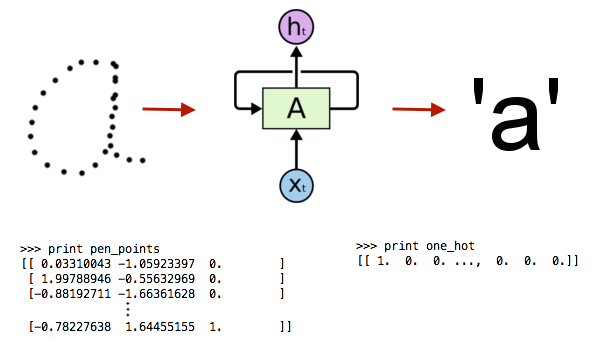
Ok, that is a tough challenge but it can be done using out-of-the-box sequential models such as recurrent neural networks (RNNs). A much more difficult challenge is to reverse the process, ie. to train a model that takes the letter ‘a’ as an input and produces a series of points that we can connect to make the letter ‘a.’
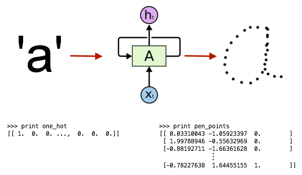
In order to make this happen, we’ll start with a recurrent neural network structure and then add some bells and whistles.
A beast of a model
It’s easy to think of the Graves handwriting model is as three separate models. Each of these models can be trained using gradient backpropagation, so we basically stack them on top of each other like Legos and then train the whole beast from end-to-end. I’ll describe each model in turn and give an intuition for how they work together to generate handwriting.
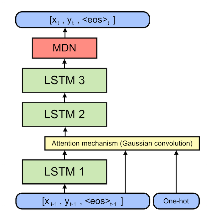
The Long Short-Term Memory (LSTM) Cell. At the core of the Graves handwriting model are three Long Short-Term Memory (LSTM) Recurrent Neural Networks (RNNs). We could just as easily have used Gated Recurrent Units (GRUs), Recurrent Highway Networks (RHNs), or some other seq2seq cell. TensorFlow provides a built-in API for these models so it doesn’t really matter. If you don’t know what recurrent neural networks or LSTMs are, read this post to see how they work and this post to see what they can do.
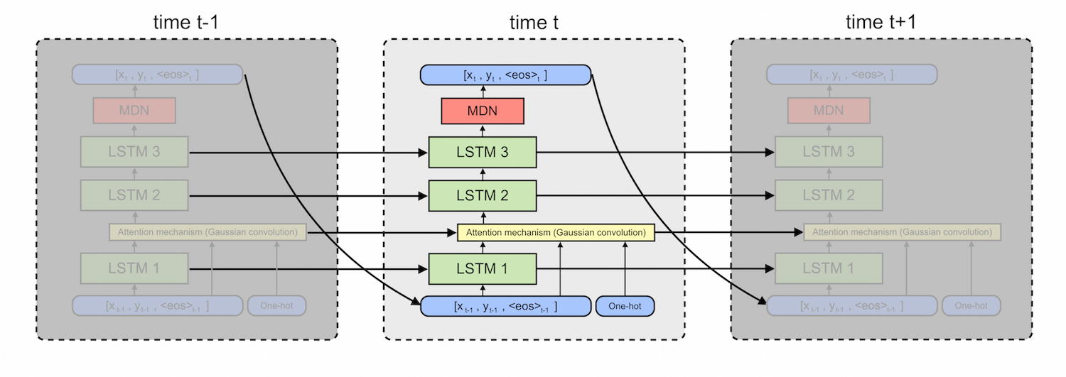
These networks use a differentiable form of memory to keep track of time-dependent patterns in data. LSTMs, for example, use three different tensors to perform ‘erase’, ‘write’, and ‘read’ operations on a ‘memory’ tensor: the \(f\), \(i\), \(o\), and \(C\) tensors respectively (more on this). For the purposes of this post, just remember that RNNs are extremely good at modeling sequential data.
The Mixture Density Network (MDN). Think of Mixture Density Networks as neural networks which can measure their own uncertainty. Their output parameters are \(\mu\), \(\sigma\), and \(\rho\) for several multivariate Gaussian components. They also estimate a parameter \(\pi\) for each of these distributions. Think of \(\pi\) as the probability that the output value was drawn from that particular component’s distribution. Last year, I wrote an Jupyter notebook about MDNs.
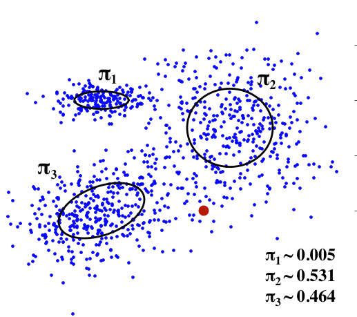
Since MDNs parameterize probability distributions, they are a great way to capture randomness in the data. In the handwriting model, the MDN learns to how messy or unpredictable to make different parts of handwriting. For example, the MDN will choose Gaussian with diffuse shapes at the beginning of strokes and Gaussians with peaky shapes in the middle of strokes.
The Attention Mechanism. Imagine that we want our model to write ‘You know nothing Jon Snow.’ In order to get the information about which characters make up this sentence, the model uses a differentiable attention mechanism. In technical terms, it is a Gaussian convolution over a one-hot ascii encoding. Think of this convolution operation as a soft window through which the handwriting model can look at a small subset of characters, ie. the letters ‘kn’ in the word ‘know’. Since all the parameters of this window are differentiable, the model learns to shift the window from character to character as it writes them
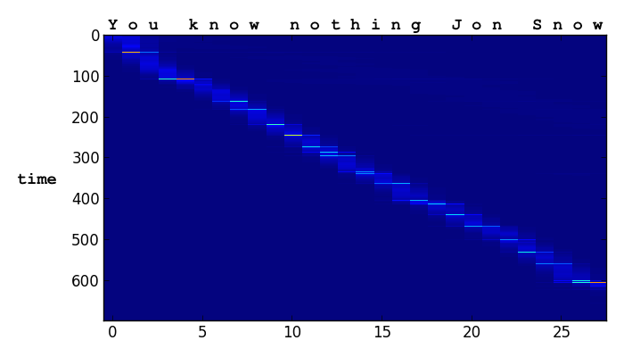
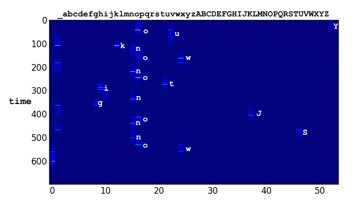
The model learns to control the window parameters remarkably well. For example, the bright stripes in the first plot are the model’s way of encoding the end of a pen stroke. We never hard-coded this behavior!
Results
It works! After a couple hours on a Tesla K40 GPU, the model generates legible letters and after a day or so it writes sentences with only a few small errors. Even though most of the training sequences were 256 points long, I was able to sample sequences of up to 750.


Since the model’s MDN cap predicts the pen’s \((x,y)\) coordinates by drawing them from a Gaussian distribution, we can modify that distribution to make the handwriting cleaner or messier. I followed Alex Graves’ example by introducing a ‘bias’ term \(b\) which redefines the \(\pi\) and \(\sigma\) parameters according to
\[\sigma^{j}_{t} = \exp \left( \hat \sigma (1+b) \right)\] \[\pi^{j}_{t} = \frac{ \exp \left( \hat \pi (1+b) \right) } { \sum_{j'=1}^{M} \exp \left( \hat \pi (1+b) \right) }\]To better understand what is happening here, check out my Jupyter notebook or the original paper. Below are results for \(b={0.5,0.75,1.0}\)


The Lego Effect
Deep learning used to be divided neatly according to algorithms. There were convolutional neural networks (ConvNets) for image recognition, RNNs for sequence analysis, and Deep-Q or Policy Gradient Networks for Reinforcement Learning. Some of the most exciting papers in the past year combine several of these algorithms in a single differentiable model.
The Lego Effect is a new trend of stacking together several differentiable models and training them all end-to-end so that each solves a subset of the task
The Graves handwriting model is one of the first examples of the Lego Effect. As I explained above, it’s actually a combination of three different types of models. The RNN cell learns to reproduce sequences of pen points, the MDN models randomness and style in the handwriting, and the attention mechanism tells the model what to write.
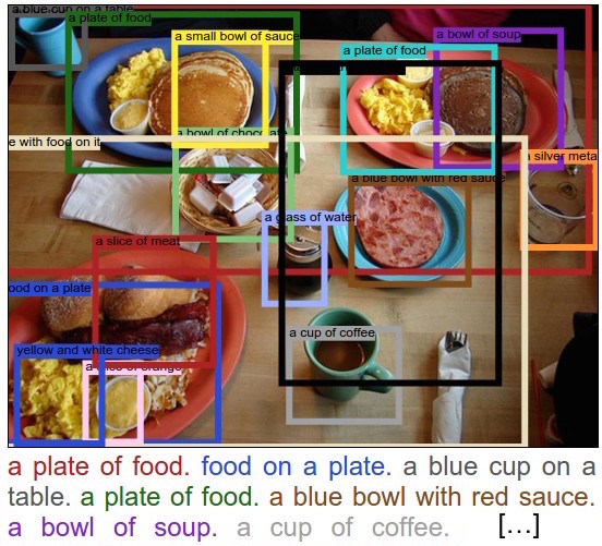
There are many other examples of the Lego Effect in the wild. Andrej Karpathy and Justin Johnson combined ConvNets with an LSTM to generate image captions. AI researchers regularly use ConvNets in their reinforcement learning models to solve vision-based games like Atari Breakout. Alex Graves and some other DeepMind researchers combined ConvNets with policy gradients in Recurrent Models of Visual Attention to do gradient-based training on a network which makes non-differentiable decisions.
These sorts of papers will only become more common in coming months. One area of rapid research which promises to benefit from the Lego Effect is differentiable long term memory. Several well-established models have short term memory (LSTMs, Gated Recurrent Units (GRUs), Recurrent Highway Networks) but only a few research-only models (Neural Turing Machines, Hierarchical Memory Networks) have the neural equivalent of a hard drive. The fact is that trainable long term memory is really tough to implement! There are some early signs of success in this area that use the Lego Effect. One really exciting paper, Reinforcement Learning Neural Turing Machines combines reinformement learning, recurrent networks, and a big bag of DL tricks to tackle the challenge.
Closing thoughts
Deep learning never started out as a way to generate handwriting. The fact that I was able to achieve state of the art in this task after only a few slight adjustments to an LSTM is what has made the field so explosive and successful. The strength of deep learning models is their generality. For example, by simply increasing the number of parameters and changing my training data, I could turn this model into a text-to-speech generator. The possibilities are limitless.
I hope this project gives you a sense of why deep learning is both extremely cool and brimming with potential. As a scientist by training, I see deep learning as a powerful tool for scientific discovery.
