The Art of Regularization

Regularization seems fairly insignificant at first glance but it has a huge impact on deep models. I’ll use a one-layer neural network trained on the MNIST dataset to give an intuition for how common regularization techniques affect learning.

Disclaimer (January 2018): This post was written when I was still studying the basics of ML. There are no errors to the best of my knowledge. But take some of the intuitions with a grain of salt.

MNIST Classification

MNIST training samples

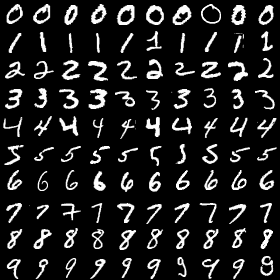
The basic idea here is to train a learning model to classify 28x28 images of handwritten digits (0-9). The dataset is relatively small (60k training examples) so it’s a classic benchmark for evaluating small models. TensorFlow provides a really simple API for loading the training data:

import tensorflow as tf
from tensorflow.examples.tutorials.mnist import input_data
mnist = input_data.read_data_sets('MNIST_data', one_hot=True)

batch = mnist.train.next_batch(batch_size)

Now batch[0] holds the training data and batch[1] holds the training labels. Making the model itself is really easy as well. For a fully-connected model without any regularization, we simply write:

x = tf.placeholder(tf.float32, shape=[None, xlen], name="x") # xlen is 28x28 = 784
y_ = tf.placeholder(tf.float32, shape=[None, ylen], name="y_") # ylen is 10

W = tf.get_variable("W", shape=[xlen,ylen])
output = tf.nn.softmax(tf.matmul(x, W)) # no bias because meh

The full code is available on GitHub. I trained each model for 150,000 interations (well beyond convergence) to accentuate the differences between regularization methods.

Visualizing regularization

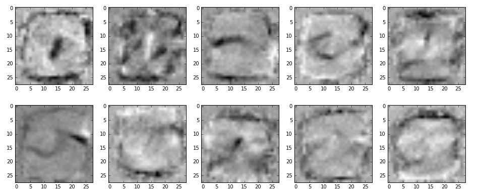
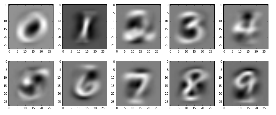
Since the model uses a 784x10 matrix of weights to map pixels to the probabilities that they represent a given digit, we can visualize which pixels are the most important for predicting a given digit. For example, to visualize which pixels are the most important for predicting the digit ‘0’, we would take the first column of the weight matrix and reshape it into a 28x28 image.

No regularization

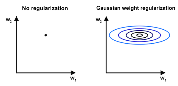
Provided the dataset is small, the model can easily overfit by making the magnitudes of some weights very large.

# no additional code

No regularization: these 'weight images' have a salt-and-pepper texture which suggests overfitting. Even so, the shadows of each of the digits are clearly visible

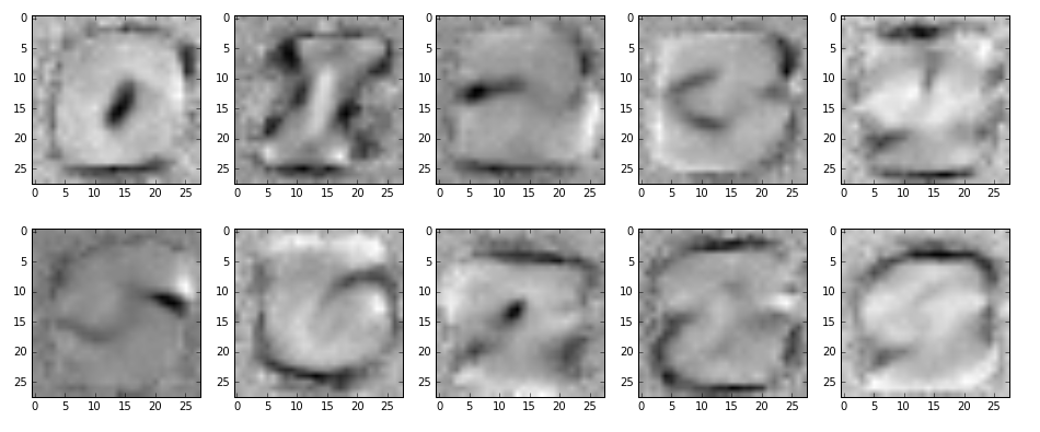
Dropout

At each training step, dropout clamps some weights to 0, effectively stopping the flow of information through these connections. This forces the model to distribute computations across the entire network and prevents it from depending heavily on a subset features. In the MNIST example, dropout has a smoothing effect on the weights

x = tf.nn.dropout(x, 0.5)

Dropout: these 'weight images' are much smoother because dropout prevents the model from placing too much trust in any one of its input features.

Gaussian Weight Regularization

The idea here is that some uncertainty is associated with every weight in the model. Weights exist in weight space not as points but as probability distributions (see below). Making a conditional independence assumption and choosing to draw a Gaussian distribution, we can represent each weight using a \(\mu\) and a \(\sigma\). Alex Graves indroduced used this concept in his adaptive weight noise poster and it also appears to be a fundamental idea in Variational Bayes models.

How to represent an optimal point in weight space

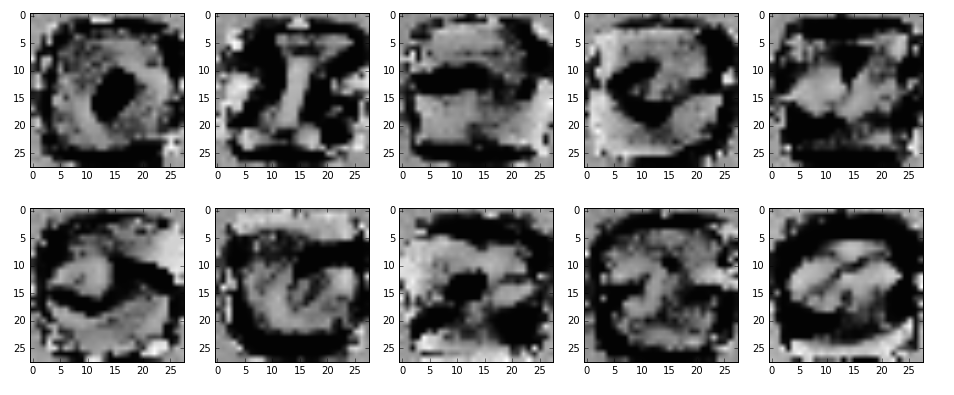
In the process of learning all this, I devised my own method for estimating \(\mu\) and a \(\sigma\). I’m not sure how to interpret the result theoretically but I thought I’d include it because 1) the weights look far different from those of the other models 2) the test accuracy is still quite high (91.5%).

S_hat = tf.get_variable("S_hat", shape=[xlen,ylen], initializer=init)
S = tf.exp(S_hat) # make sure sigma matrix is positive

mu = tf.get_variable("mu", shape=[xlen,ylen], initializer=init)
W = gaussian(noise_source, mu, S) # draw each weight from a Gaussian distribution

Gaussian weight regularization: these 'weight images' are really different but the model approaches the same training accuracy as the unregularized version.

L2 regularization

L2 regularization penalizes weights with large magnitudes. Large weights are the most obvious symptom of overfitting, so it’s an obvious fix. It’s less obvious that L2 regularization actually has a Bayesian interpretation: since we initialize weights to very small values and L2 regression keeps these values small, we’re actually biasing the model towards the prior.

loss = tf.nn.l2_loss( y_ - output ) / (ylen*batch_size) + \
		 sum(tf.get_collection(tf.GraphKeys.REGULARIZATION_LOSSES))

L2 regularization: these 'weight images' are very smooth and the digits are clear. Though the model has a better representation of how each digit appears, the test accuracy is low because messy/unusual examples don't fit the template well.

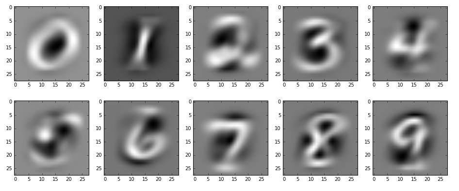
Weight normalization

Normalizing the weight matrix is another way of keeping weights close to zero so it behaves similarly to L2 regularization. However, this form of regularization is not equivalent to L2 regularization and may behave differently in wider/deeper models.

W = tf.nn.l2_normalize(W, [0,1])

Weight normalization: it's interesting to note that normalizing the weight matrix has the same effect here as L2 regularization

Comparison

\(^1\)Accuracy doesn’t matter much at this stage because it changes dramatically as we alter hyperparameters and model width/depth. In fact, I deliberately made the hyperparameters very large to accentuate differences between each of the techniques. One thing to note is that Gaussian weight regularization achieves nearly the same accuracy as the unregularized model even though its weights are very different.

\(^2\)Since Gaussian weight regularization solves for a \(\mu\) and \(\sigma\) for every single parameter, it ends up optimizing twice as many parameters which also roughly doubles runtime.

\(^3\)L2 regularization and weight normalization are designed to keep all weights small, which is why the min/max values are small. Meanwhile, Gaussian weight regularization produces an exclusively positive weight matrix because the Gaussian function is always positive.

Closing thoughts

Regularization matters! Not only is it a way of preventing overfitting; it’s also the easiest way to control what a model learns. For further reading on the subject, check out these slides.

We can expect that dropout will smooth out multilayer networks in the same way it does here. Although L2 regularization and weight normalization are very different computations, the qualititive similarity we discovered here probably extends to larger models. Gaussian weight regularization, finally, offers a promising avenue for further investigation.