Taming Wave Functions with Neural Networks

NOTE: This is a repost from an article I wrote for Quantum Frontiers, the blog of the Institute for Quantum Information and Matter at Caltech

The wave function is essential to most calculations in quantum mechanics, and yet it’s a difficult beast to tame. Can neural networks help?

Wave functions in the wild

”\(\psi\) is a monolithic mathematical quantity that contains all the information on a quantum state, be it a single particle or a complex molecule.” – Carleo and Troyer, Science

The wave function, \(\psi\) , is a mixed blessing. At first, it causes unsuspecting undergrads (me) some angst via the Schrodinger’s cat paradox. This angst morphs into full-fledged panic when they encounter concepts such as nonlocality and Bell’s theorem (which, by the way, is surprisingly hard to verify experimentally). The real trouble with \(\psi\), though, is that it grows exponentially with the number of entangled particles in a system. We couldn’t even hope to write the wavefunction of 100 entangled particles, much less perform computations on it…but there’s a lot to gain from doing just that.

The thing is, we (a couple of luckless physicists) love \(\psi\) . Manipulating wave functions can give us ultra-precise timekeeping, secure encryption, and polynomial-time factoring of integers (read: break RSA). Harnessing quantum effects can also produce better machine learning, better physics simulations, and even quantum teleportation.

Taming the beast

Though \(\psi\) grows exponentially with the number of particles in a system, most physical wave functions can be described with a lot less information. Two algorithms for doing this are the Density Matrix Renormalization Group (DMRG) and Quantum Monte Carlo (QMC).

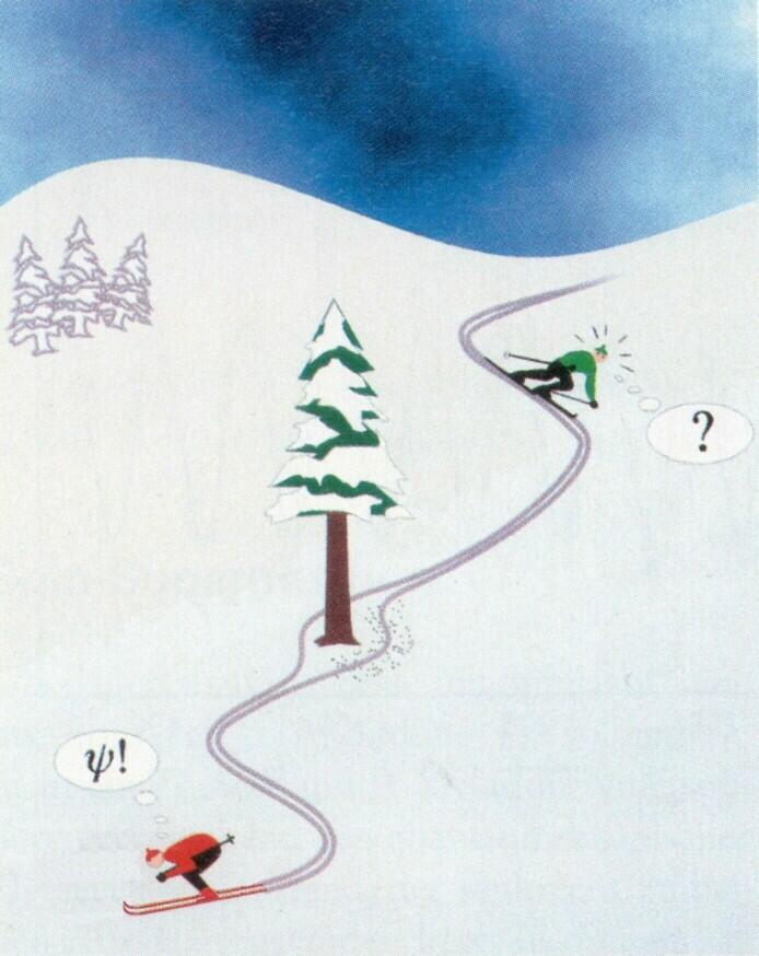
Density Matrix Renormalization Group (DMRG). Imagine we want to learn about trees, but studying a full-grown, 50-foot tall tree in the lab is too unwieldy. One idea is to keep the tree small, like a bonsai tree. DMRG is an algorithm which, like a bonsai gardener, prunes the wave function while preserving its most important components. It produces a compressed version of the wave function called a Matrix Product State (MPS). One issue with DMRG is that it doesn’t extend particularly well to 2D and 3D systems.

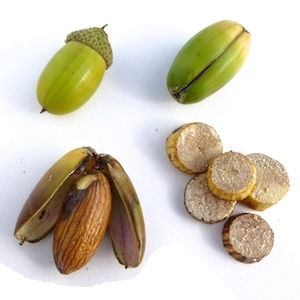
Quantum Monte Carlo (QMC). Another way to study the concept of “tree” in a lab (bear with me on this metaphor) would be to study a bunch of leaf, seed, and bark samples. Quantum Monte Carlo algorithms do this with wave functions, taking “samples” of a wave function (pure states) and using the properties and frequencies of these samples to build a picture of the wave function as a whole. The difficulty with QMC is that it treats the wave function as a black box. We might ask, “how does flipping the spin of the third electron affect the total energy?” and QMC wouldn’t have much of a physical answer.

Brains \(\gg\) Brawn

A schema of the Neural Quantum State (NQS) model introduced By Carleo and Troyer. The model has a Restricted Boltzman Machine (RBM) architecture. Increasing M, the number of units in the hidden layer, increases accuracy.

Neural Quantum States (NQS). Some state spaces are far too large for even Monte Carlo to sample adequately. Suppose now we’re studying a forest full of different species of trees. If one type of tree vastly outnumbers the others, choosing samples from random trees isn’t an efficient way to map biodiversity. Somehow, we need to make the sampling process “smarter”. Last year, Google DeepMind used a technique called deep reinforcement learning to do just that – and achieved fame for defeating the world champion human Go player.

A recent Science paper by Carleo and Troyer (2017) used the same technique to make QMC “smarter” and effectively compress wave functions with neural networks. This approach, called “Neural Quantum States (NQS)”, produced several state-of-the-art results.

A schema of the neural network model I used to obtain MPS coefficients. The Hamiltonian I'm using is a Heisenberg Hamiltonain plus extra coupling terms (see my thesis for details). Colors denote the magnitudes of scalar matrix elements.

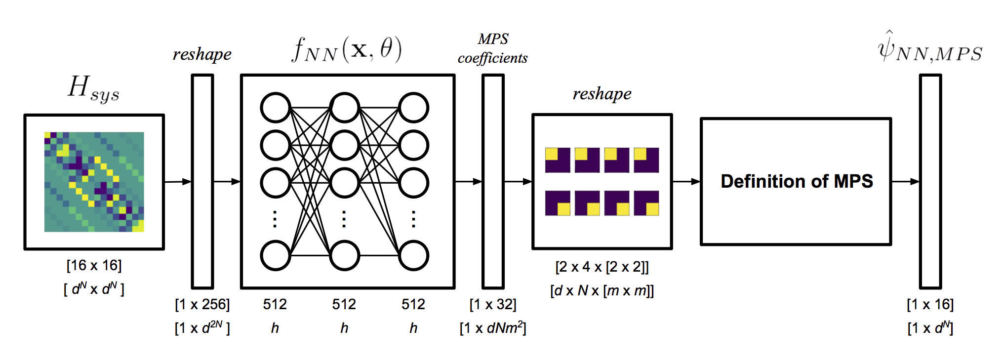
My thesis. My undergraduate thesis, which I conducted under fearless Professor James Whitfield of Dartmouth College, centered upon much the same idea. In fact, I had to abandon some of my initial work after reading the NQS paper. I then focused on using machine learning techniques to obtain MPS coefficients. Like Carleo and Troyer, I used neural networks to approximate \psi . Unlike Carleo and Troyer, I trained my model to output a set of Matrix Product State coefficients which have physical meaning (MPS coefficients always correspond to a certain state and site, e.g. “spin up, electron number 3”).

A word about MPS. I should quickly explain what, exactly, a Matrix Product State is. Check out the equation above, which is the definition of MPS. The idea is to multiply a set of matrices, \(A\) together and take the trace of the result. Each \(A\) matrix corresponds to a particular site, \(A[n]\), (e.g. “electron 3”) and a particular state, \(A^{s_i}\) (e.g. “spin \(\frac{1}{2}\)”). Each of the values obtained from the trace operation becomes a single coefficient of \(\psi\), corresponding to a particular state \(\lvert s_1, \dots s_N \rangle\).

Does it work?

Yes – for small systems. In my thesis, I considered a toy system of 4 spin-\frac{1}{2} particles interacting via the Heisenberg Hamiltonian. Solving this system is not difficult so I was able to focus on fitting the two disparate parts – machine learning and Matrix Product States – together.

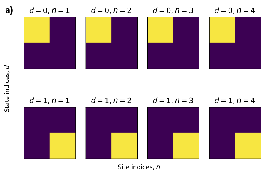
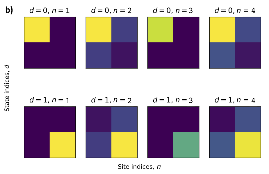
Success! My model solved for ground states with arbitrary precision. Even more interestingly, I used it to automatically obtain MPS coefficients. Shown below, for example, is a visualization of my model’s coefficients for the GHZ state, compared with coefficients taken from the literature.

A visual comparison of a 4-site Matrix Product State for the GHZ state a) listed in the literature b) obtained from my neural network model.

Limitations. The careful reader might point out that, according to the schema of my model (above), I still have to write out the full wave function. To scale my model up, I instead trained it variationally over a subspace of the Hamiltonian (just as the authors of the NQS paper did). Results are decent for larger (10-20 particle) systems, but the training itself is still unstable. I’ll finish ironing out the details soon, so keep an eye on arXiv¹ :).

Looking beyond fundamental research

A quantum computer developed by Joint Quantum Institute, U. Maryland.

Quantum computing is a field that’s poised to take on commercial relevance. Taming the wave function is one of the big hurdles we need to clear before this happens. Hopefully my findings will have a small role to play in making this happen.

On a more personal note, thank you for reading about my work. As a recent undergrad, I’m still new to research and I’d love to hear constructive comments or criticisms. If you found this post interesting, check out my research blog.