Hamiltonian Neural Networks

Figure 1: Instead of crafting a Hamiltonian by hand, we parameterize it with a neural network and then learn it directly from data. The variables q and p correspond to position and momentum coordinates. As there is no friction, the baseline's inward spiral is due to model errors. By comparison, the Hamiltonian Neural Network learns to exactly conserve an energy-like quantity.

The Wisdom of Learning Invariant Quantities

It’s remarkable that we ever have an “ordinary day.” If we were to sit down and catalogue all of our experiences – the flavors of our sandwich, the quality of the sunlight, or the texture of our cat’s fur – no day would look like any other. The stew of sensory information would be simply overwhelming.

The only way to make sense of our complicated day-to-day experiences is to focus on the things that don’t change. The invariants. The conserved quantities. Over time, we pick up on these things and use them as anchors or reference points for our sense of reality. Our sandwich tastes different…maybe the bread is stale. The cat doesn’t feel as soft as usual…maybe it needs a bath. It’s beneficial to understand what does not vary in order to make sense of what does.

This is a common theme in physics. Physicists start with a small set of “invariant quantities” such as total energy, total momentum, and (sometimes) total mass. Then they use these invariances to predict the dynamics of a system. “If energy is conserved,” they might say, “when I throw a ball upwards, it will return to my hand with the same speed as when it left.”

But these common-sense rules can be difficult to learn straight from data. On tasks such as video classification, reinforcement learning, or robotic dexterity, machine learning researchers train neural networks on millions of examples. And yet, even after seeing all of these examples, neural networks don’t learn exact conservation laws. The best they can do is gradually improve their approximations.

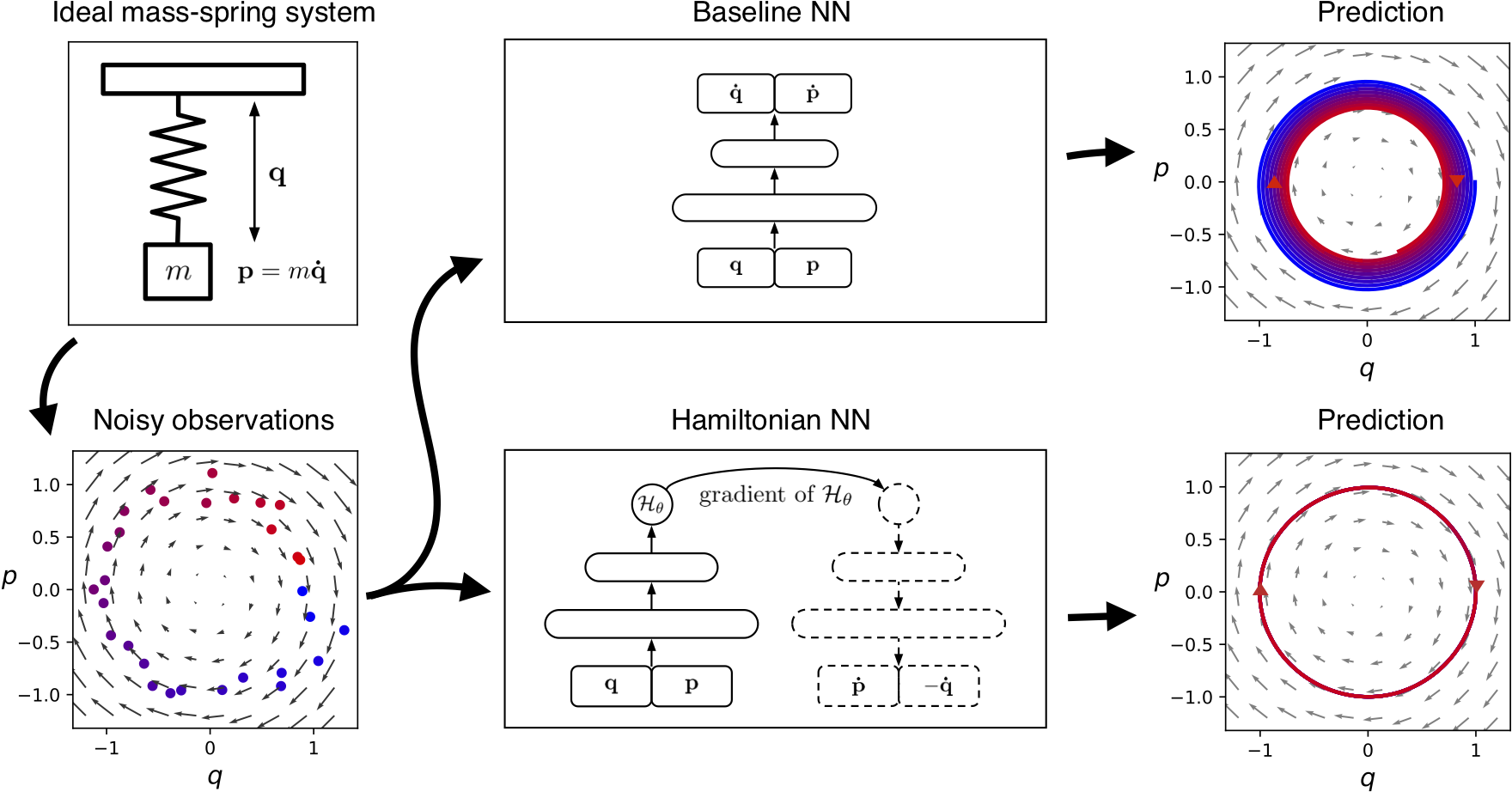
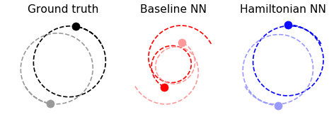
As an example, consider the ideal mass-spring system shown in Figure 1. Here the total energy of the system is being conserved. More specifically, a quantity proportional to \(q^2+p^2\) is being conserved, where \(q\) is the position and \(p\) is the momentum of the mass. The baseline neural network learns an approximation of this conservation law, and yet the approximation is imperfect enough that a forward simulation of the system drifts slowly to a different energy state. Can we design a model that doesn’t drift?

Hamiltonian Neural Networks

It turns out we can. Drawing inspiration from Hamiltonian mechanics, a branch of physics concerned with conservation laws and invariances, we define Hamiltonian Neural Networks, or HNNs. By construction, these models learn conservation laws from data. We’ll show that they have some major advantages over regular neural networks on a variety of physics problems.

Play

Figure 3: Two bodies interact via a gravitational force. The dynamics of the baseline model do not conserve total energy and quickly diverge from ground truth. Meanwhile, the HNN learns to conserve a quantity that is close to total energy. This makes its predicted trajectories more stable.

We begin with an equation called the Hamiltonian, which relates the state of a system to some conserved quantity (usually energy) and lets us simulate how the system changes with time. Physicists generally use domain-specific knowledge to find this equation, but here we try a different approach: Instead of crafting Hamiltonians by hand, we parameterize them with neural networks and then learn them directly from data.

Related work. A variety of previous works have sought to endow neural networks with intuitive physics priors. Some of these works were domain-specific: they solved problems in molecular dynamics¹, quantum mechanics², or robotics³. Others, such as Interaction Networks⁴, were meant to be fully general. A common pattern among these works, is that none of them showed how to learn invariant quantities. Schmidt and Lipson⁵ did tackle this challenge, but whereas they used a genetic algorithm to search over a space of mathematical expressions, in this work we train a neural network with gradient descent.

A Quick Tour of Hamiltonian Mechanics

In order to situate our model in the proper context, we will use this section to review the basics of Hamiltonian mechanics.

History. William Hamilton introduced Hamiltonian mechanics in the 19th century as a mathematical reformulation of classical mechanics. Its original purpose was to express classical mechanics in a more unified and general manner. Over time, though, scientists have applied it to nearly every area of physics.

Theory. In Hamiltonian mechanics, we begin with a set of coordinates \((\mathbf{q},\mathbf{p})\). Usually, \(\mathbf{q}=(q_1,…,q_N)\) represents the positions of a set of objects whereas \(\mathbf{p}=(p_1,…, p_N)\) denotes their momentum. Note how this gives us \(N\) coordinate pairs \((q_1,p_1)…(q_N,p_N)\). Taken together, they offer a complete description of the system. Next, we define a scalar function, \(\mathcal{H}(\mathbf{q},\mathbf{p})\) called the Hamiltonian so that

This equation tells us that moving coordinates in the direction \(\mathbf{S_{\mathcal{H}}} = \big(\frac{\partial \mathcal{H}}{\partial \mathbf{p}}, -\frac{\partial \mathcal{H}}{\partial \mathbf{q}} \big)\) gives us the time evolution of the coordinates. We can think of \(\mathbf{S}\) as a vector field over the inputs of \(\mathcal{H}\). In fact, it is a special kind of vector called a “symplectic gradient’’. Whereas moving in the direction of the gradient of \(\mathcal{H}\) changes the output as quickly as possible, moving in the direction of the symplectic gradient keeps the output exactly constant. Hamilton used this mathematical framework to relate the position and momentum vectors \((\mathbf{q},\mathbf{p})\) of a system to its total energy \( E_{tot}=\mathcal{H}(\mathbf{q},\mathbf{p}) \). Then, he obtained the time evolution of the system by integrating this field according to

Uses. This is a powerful approach because it works for almost any system where the total energy is conserved. Like Newtonian mechanics, it can predict the motion of a mass-spring system or a single pendulum. But its true strengths become apparent when we tackle large and/or chaotic systems like quantum many-body problems, fluid simulations, and celestial orbitals. Hamiltonian mechanics gives us a common language to describe these systems as well as set of first-order differential equations for their dynamics.

Overview. To summarize, Hamiltonian mechanics is a tool for modeling large and chaotic physical systems. It’s useful because it generalizes to almost any field of physics and can handle systems that are large and chaotic. The general recipe for applying Hamiltonian mechanics to a problem is:

1. Choose a set of coordinates that describe the state of a system⁶. A common choice is position and momentum \((\mathbf{q},\mathbf{p})\).
2. Write the total energy of the system as a function of those coordinates⁷. This equation is called the Hamiltonian.
3. Compute the partial derivatives of the Hamiltonian w.r.t. the coordinates. Then use Hamilton’s equations (Equation 1) to find the time derivatives of the system.
4. Integrate the time derivatives to predict the state of the system at some time in the future (Equation 2).

Learning Hamiltonians from Data

Let’s use neural networks to learn Hamiltonians from data. In particular, let’s consider a dataset that consists of coordinate trajectories through time: either directly (the actual \((\mathbf{q},\mathbf{p})\) coordinates) or indirectly (pixel images that contain \((\mathbf{q},\mathbf{p})\) information). Also, let’s suppose that we’ve parameterized a Hamiltonian with neural network parameters \(\theta\). The first thing to notice is that we can rewrite Equation \eqref{eq:eqn1} so that both terms are on the left side:

Since we know that the function \(\mathcal{H}\) is a Hamiltonian when both of these terms go to zero, we can rewrite it as a solution to the following minimization objective:

Now this expression is beginning to look like the \(\mathcal{L_2}\) loss function used in supervised learning. The \(\mathcal{L_2}\) loss term usually takes the form \(\big \Vert y - f_{\theta}(x) \big \Vert^2 \) where \(x\) is the input and \(y\) is the target. The key difference is that here we are minimizing something of the form \( \big \Vert y - \frac{\partial f_{\theta}(x)}{\partial x} \big \Vert^2 \). In other words, we are optimizing the gradient of a neural network.

Figure 4: Schema of the Baseline and HNN models. The Baseline NN in the figure above represents the supervised learning approach to modeling the time derivatives of (q, p). In both cases, the inputs are the coordinates of the system and the targets are their time derivatives.

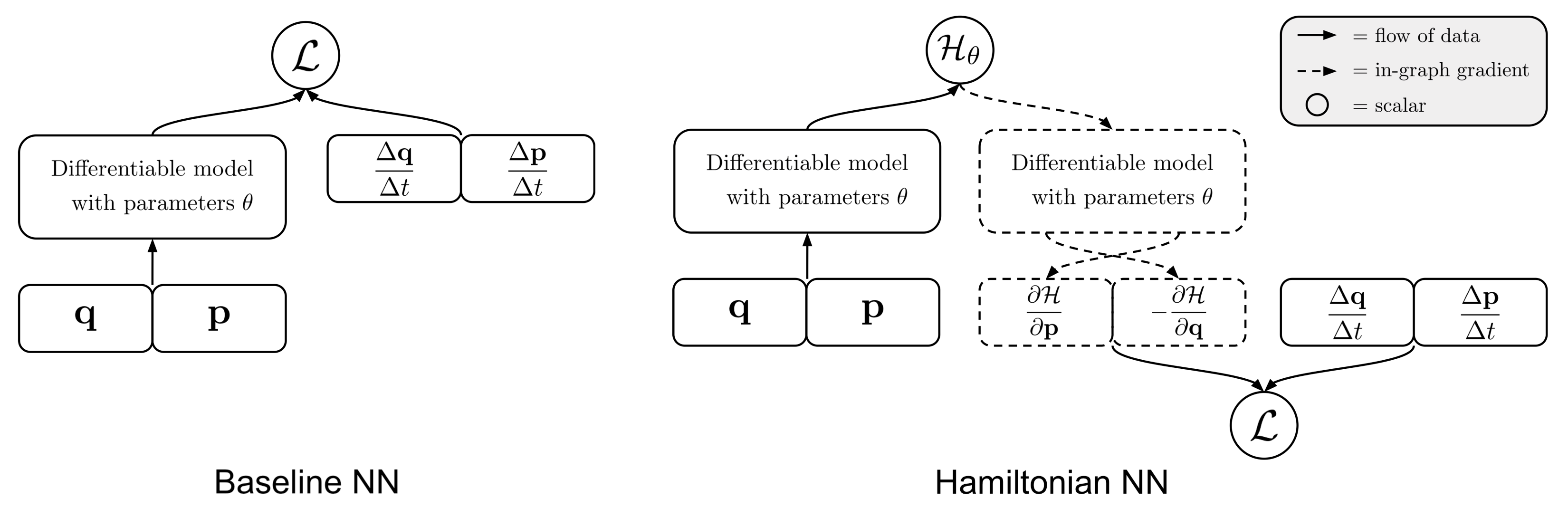
There are not many previous works that optimize the gradients of a neural network. Work by Schmidt and Lipson⁵ uses a loss function of this form, but they do not use it to optimize a neural network. Wang et al.⁸ optimize the gradients of a neural network, but not for the purpose of learning Hamiltonians. But not only is this technique possible; we also found that it works reasonably well.

Results on simple tasks. We trained an HNN and a baseline model on three simple physics tasks. You can explore the setup and results for each of these tasks in Figure 5. Generally speaking, the HNN trained about as easily as the baseline model and produced better results. In order to predict dynamics, we integrated our models using scipy.integrate.solve_ivp and set the error tolerance to \(10^{-9}\)

Next task

Figure 5: In Task 1, we trained the HNN on data from a simulated mass-spring system. The dynamics of this system were perfectly linear, making this the simplest system we considered. Notice how the HNN learns to conserve a quantity very similar to the total energy of the system.

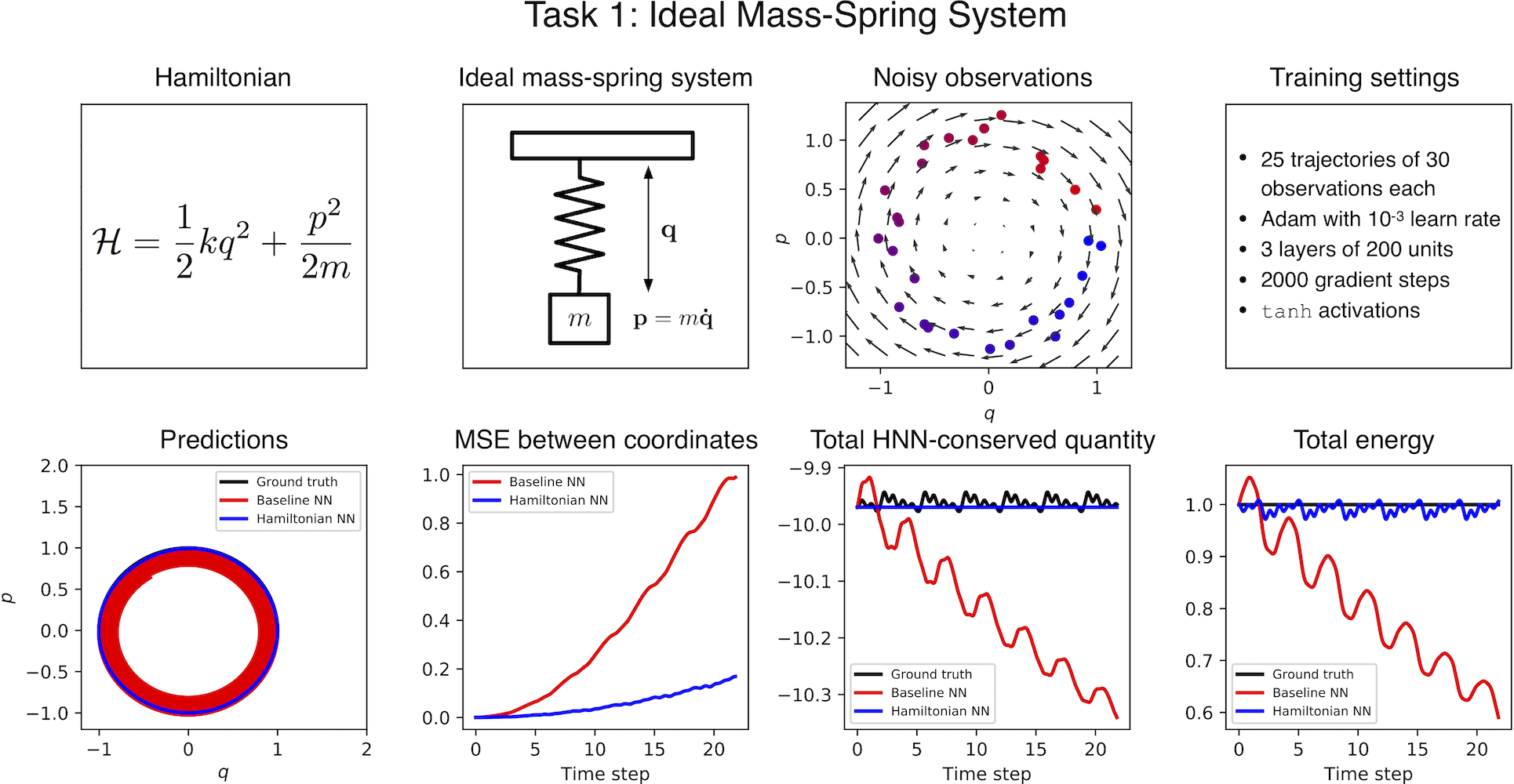
What is the HNN conserving? It’s worth noting that the quantity conserved by the HNN is not equivalent to the total energy; rather, it’s something very close to the total energy. The last two plots in Figure 5 provide a useful comparison between the HNN-conserved quantity and the total energy. Looking closely at the spacing of the \(y\) axes, you can see that the HNN-conserved quantity has the same scale as total energy, but differs by a constant factor. Since energy is a relative quantity, this is perfectly acceptable⁹.

Modeling Larger Systems

Having established baselines on a few simple tasks, our next step was to tackle a larger system involving more than one pair of \((\mathbf{q},\mathbf{p})\) coordinates. One well-studied problem that fits this description is the \(N\)-body problem, which requires \(2N\) pairs, where \(N\) is the number of bodies.

Figure 6: (Left) Two bodies interact via a gravitational force. The dynamics of the baseline model do not conserve total energy and quickly diverge from ground truth. The HNN, meanwhile, approximately conserves total energy and accrues a small amount of error after one full orbit. (Right) Three bodies interact via a gravitational force. This system is chaotic and has a large dynamic range. While neither of our models achieves good performance on this dataset, the HNN substantially outperforms the baseline and shows promising generalization.

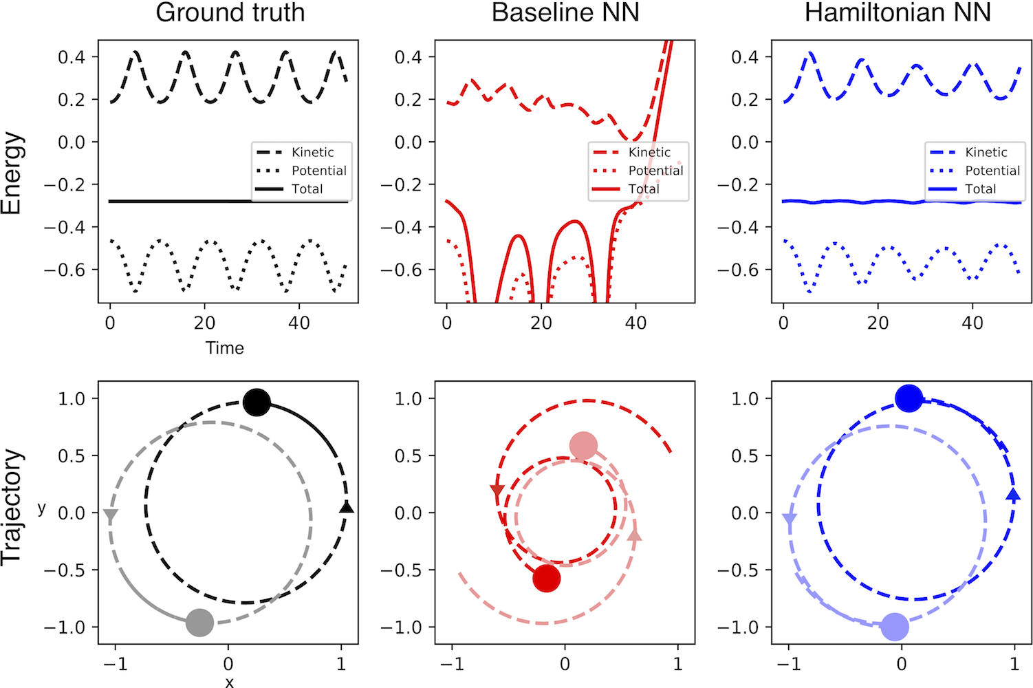
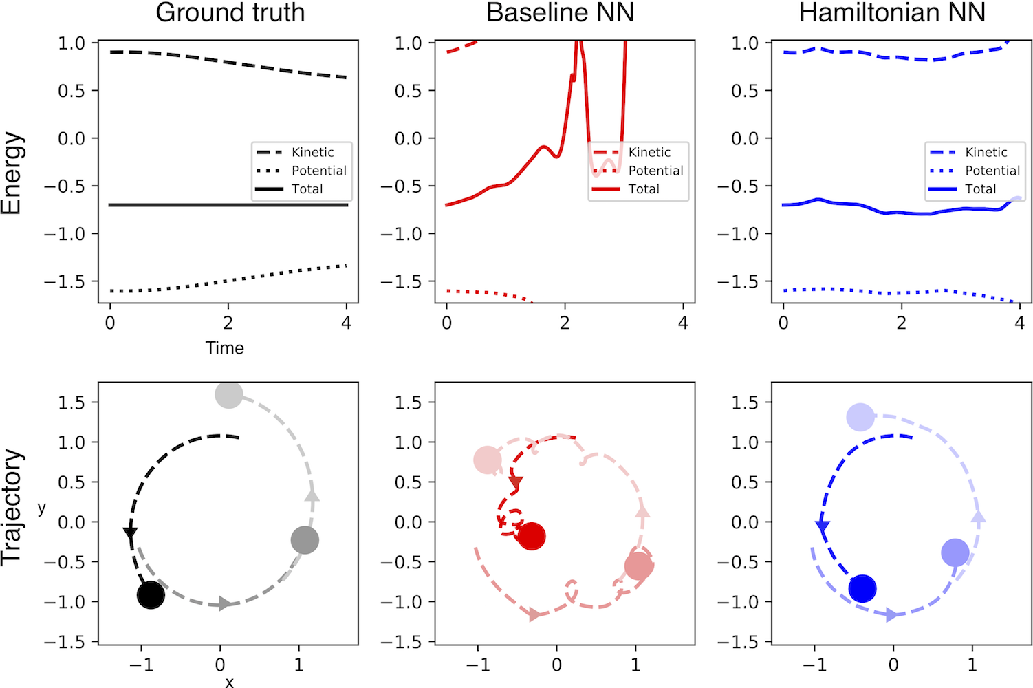
Figure 6 shows qualitative results for systems with two and three bodies. We suspect that neither model converged to a good solution on the three body task because of the large dynamic range of the dataset; we hope to fix this in future work.

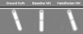
Learning a Hamiltonian from Pixels

One of the key strengths of neural networks is that they can learn abstract representations directly from high-dimensional data such as pixels or words. Having trained HNN models on position and momentum coordinates, we were eager to see whether we could train them on arbitrary coordinates like the latent vectors of an autoencoder.

The Pixel Pendulum. First, we constructed a dataset of pixel observations of a pendulum by stepping through the OpenAI Gym Pendulum-v0 environment. Then we combined an autoencoder with an HNN to learn the dynamics of the system. The autoencoder would consume two adjacent frames (for velocity information) and then pass its latent codes to the HNN, which used them just as it would a set of \((\mathbf{q},\mathbf{p})\) coordinates. We trained the entire model end-to-end and found that it outperformed the baseline by a significant margin. To our knowledge this is the first instance of a Hamiltonian learned directly from pixel data!

Play

Figure 7: Predicting the dynamics of the pixel pendulum. We train an HNN and its baseline to predict dynamics in the latent space of an autoencoder. Then we project the latent trajectory back to pixel space for visualization. The baseline model rapidly decays to lower energy states whereas the HNN remains close to ground truth even after hundreds of frames.

For full disclosure, we did end up adding an auxiliary loss to the model in order to make the latent space look more like a set of canonical coordinates (see paper for details). However, this is not domain-specific and did not affect the performance of the autoencoder.

Other Mischief with HNNs

While the main purpose of HNNs is to endow neural networks with better physics priors, they have a few other nice properties. It’s worth touching on these before wrapping things up.

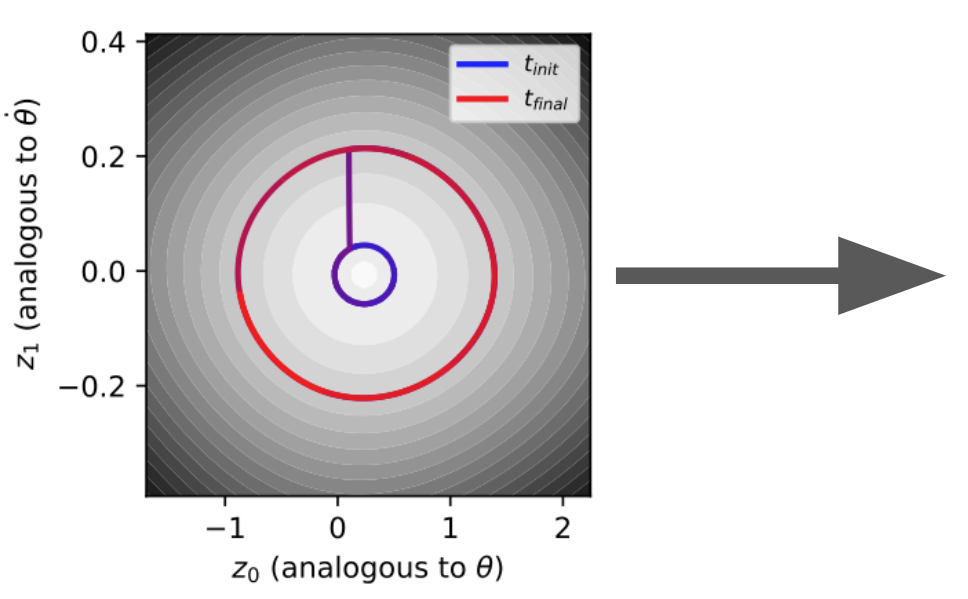
Adding and removing energy. So far, we have only integrated the symplectic gradient of the Hamiltonian. This keeps the scalar, energy-like value of \(\mathcal{H}(\mathbf{q},\mathbf{p})\) fixed. But we could just as easily follow the regular gradient of the Hamiltonian in order to increase or decrease \(\mathcal{H}\). We can even alternate between changing and conserving the energy-like value. Figure 8 shows how we can use this process to “bump” the pendulum to a higher energy level. We could imagine using this technique to answer counterfactual questions e.g. “What would have happened if we added 1 Joule of energy?””

Play

Figure 8: Visualizing integration in the latent space of the Pixel Pendulum model. We alternate between integrating the symplectic gradient at low energy (blue circle), the regular gradient (purple line), and then the symplectic gradient at higher energy (red circle).

Perfect reversibility. The HNN learns a vector field that has zero divergence. In other words, there are no sources or sinks. This means that we could integrate our model forward for an arbitrary amount of time and then run it backwards and exactly recover the original inputs. Check out the paper for more on this idea!

Closing Thoughts

Whereas Hamiltonian mechanics is an old and well-established theory, the science of deep learning is still in its infancy. Whereas Hamiltonian mechanics describes the real world from first principles, deep learning does so starting from data. We believe that Hamiltonian Neural Networks, and models like them, represent a promising way of bringing together the strengths of both approaches.

Acknowledgements

Thanks to the Google AI Residency for providing me with all the mentorship and resources that a young researcher could dare to dream of. Thanks to Nic Ford, Trevor Gale, Rapha Gontijo Lopes, Keren Gu, Ben Caine, Mark Woodward, Stephan Hoyer, and Jascha Sohl-Dickstein for insightful conversations and advice. Thanks to Jason Yosinski and Misko Dzamba for being awesome coauthors and for the informal conversations that sparked this work.

Footnotes