Scaling down Deep Learning

By any scientific standard, the Human Genome Project was enormous: it involved billions of dollars of funding, dozens of institutions, and over a decade of accelerated research. But that was only the tip of the iceberg. Long before the project began, scientists were hard at work assembling the intricate science of human genetics. And most of the time, they were not studying humans. The foundational discoveries in genetics centered on far simpler organisms such as peas, molds, fruit flies, and mice. To this day, biologists use these simpler organisms as genetic “minimal working examples” in order to save time, energy, and money. A well-designed experiment with Drosophilia, such as Feany and Bender (2000), can teach us an astonishing amount about humans.

The deep learning analogue of Drosophilia is the MNIST dataset. A large number of deep learning innovations including dropout, Adam, convolutional networks, generative adversarial networks, and variational autoencoders began life as MNIST experiments. Once these innovations proved themselves on small-scale experiments, scientists found ways to scale them to larger and more impactful applications.

They key advantage of Drosophilia and MNIST is that they dramatically accelerate the iteration cycle of exploratory research. In the case of Drosophilia, the fly’s life cycle is just a few days long and its nutritional needs are negligible. This makes it much easier to work with than mammals, especially humans. In the case of MNIST, training a strong classifier takes a few dozen lines of code, less than a minute of walltime, and negligible amounts of electricity. This is a stark contrast to state-of-the-art vision, text, and game-playing models which can take months and hundreds of thousands of dollars of electricity to train.

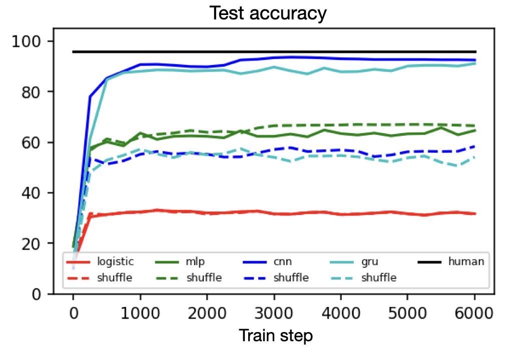
Yet in spite of its historical significance, MNIST has three notable shortcomings. First, it does a poor job of differentiating between linear, nonlinear, and translation-invariant models. For example, logistic, MLP, and CNN benchmarks obtain 94, 99+, and 99+% accuracy on it. This makes it hard to measure the contribution of a CNN’s spatial priors or to judge the relative effectiveness of different regularization schemes. Second, it is somewhat large for a toy dataset. Each input example is a 784-dimensional vector and thus it takes a non-trivial amount of computation to perform hyperparameter searches or debug a metalearning loop. Third, MNIST is hard to hack. The ideal toy dataset should be procedurally generated so that researchers can smoothly vary parameters such as background noise, translation, and resolution.

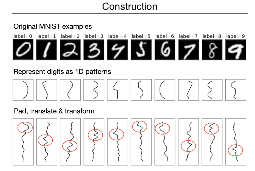
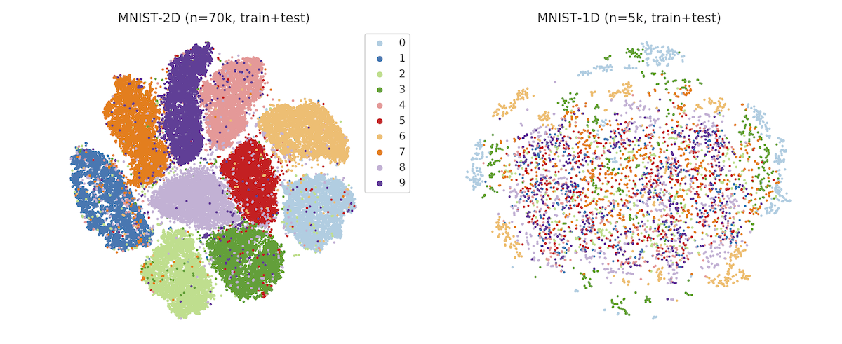
In order to address these shortcomings, we propose the MNIST-1D dataset. It is a minimalist, low-memory, and low-compute alternative to MNIST, designed for exploratory deep learning research where rapid iteration is a priority. Training examples are 20 times smaller but they are still better at measuring the difference between 1) linear and nonlinear classifiers and 2) models with and without spatial inductive biases (eg. translation invariance). The dataset is procedurally generated but still permits analogies to real-world digit classification.

Constructing the MNIST-1D dataset. Like MNIST, the classifier's objective is to determine which digit is present in the input. Unlike MNIST, each example is a one-dimensional sequence of points. To generate an example, we begin with a digit template and then randomly pad, translate, and transform it.

Visualizing the performance of common models on the MNIST-1D dataset. This dataset separates them cleanly according to whether they use nonlinear features (logistic regression vs. MLP) or whether they have spatial inductive biases (MLP vs. CNN). Humans do best of all. Best viewed with zoom.

Visualizing the MNIST and MNIST-1D datasets with tSNE. The well-defined clusters in the MNIST plot indicate that the majority of the examples are separable via a kNN classifier in pixel space. The MNIST-1D plot, meanwhile, reveals a lack of well-defined clusters which suggests that learning a nonlinear representation of the data is much more important to achieve successful classification. Thanks to Dmitry Kobak for making this plot.

Example use cases

In this section we will explore several examples of how MNIST-1D can be used to study core “science of deep learning” phenomena.

Finding lottery tickets. It is not unusual for deep learning models to have ten or even a hundred times more parameters than necessary. This overparameterization helps training but increases computational overhead. One solution is to progressively prune weights from a model during training so that the final network is just a fraction of its original size. Although this approach works, conventional wisdom holds that sparse networks do not train well from scratch. Recent work by Frankle & Carbin (2019) challenges this conventional wisdom. The authors report finding sparse subnetworks inside of larger networks that train to equivalent or even higher accuracies. These “lottery ticket” subnetworks can be found through a simple iterative procedure: train a network, prune the smallest weights, and then rewind the remaining weights to their original initializations and retrain.

Since the original paper was published, a multitude of works have sought to explain this phenomenon and then harness it on larger datasets and models. However, very few works have attempted to isolate a “minimal working example” of this effect so as to investigate it more carefully. The figure below shows that the MNIST-1D dataset not only makes this possible, but also enables us to elucidate, via carefully-controlled experiments, some of the reasons for a lottery ticket’s success. Unlike many follow-up experiments on the lottery ticket, this one took just two days of researcher time to produce. The curious reader can also reproduce these results in their browser in a few minutes.

Finding and analyzing lottery tickets. In a-b), we isolate a "minimum viable example" of the effect. Recent work by Morcos et al (2019) shows that lottery tickets can transfer between datasets. We wanted to determine whether spatial inductive biases played a role. So we performed a series of experiments: in c) we plot the asymptotic performance of a 92% sparse ticket. In d) we reverse all the 1D signals in the dataset, effectively preserving spatial structure but changing the location of individual datapoints. This is analogous to flipping an image upside down. Under this ablation, the lottery ticket continues to win.

Next, in e) we permute the indices of the 1D signal, effectively removing spatial structure from the dataset. This ablation hurts lottery ticket performance significantly more, suggesting that part of the lottery ticket's performance can be attributed to a spatial inductive bias. Finally, in f) we keep the lottery ticket sparsity structure but initialize its weights with a different random seed. Contrary to results reported in Frankle & Carbin (2019), we see that our lottery ticket continues to outperform a dense baseline, aligning well with our hypothesis that the lottery ticket mask has a spatial inductive bias. In g), we verify our hypothesis by measuring how often unmasked weights are adjacent to one another in the first layer of our model. The lottery ticket has many more adjacent weights than chance would predict, implying a local connectivity structure which helps give rise to spatial biases.

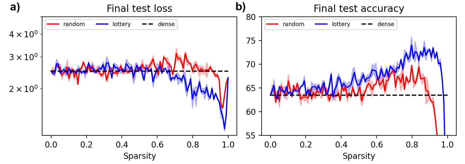
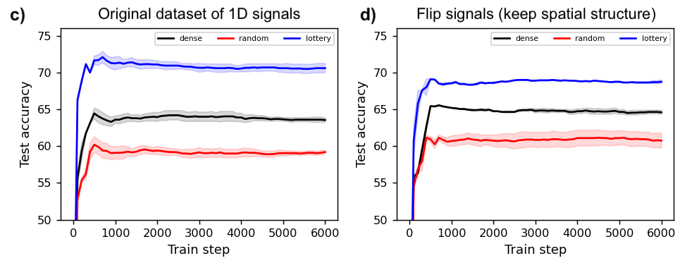
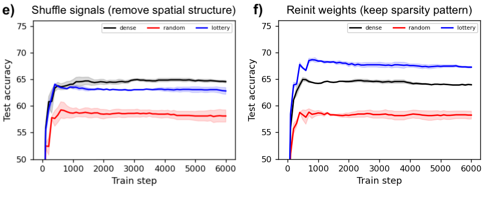
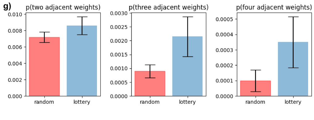
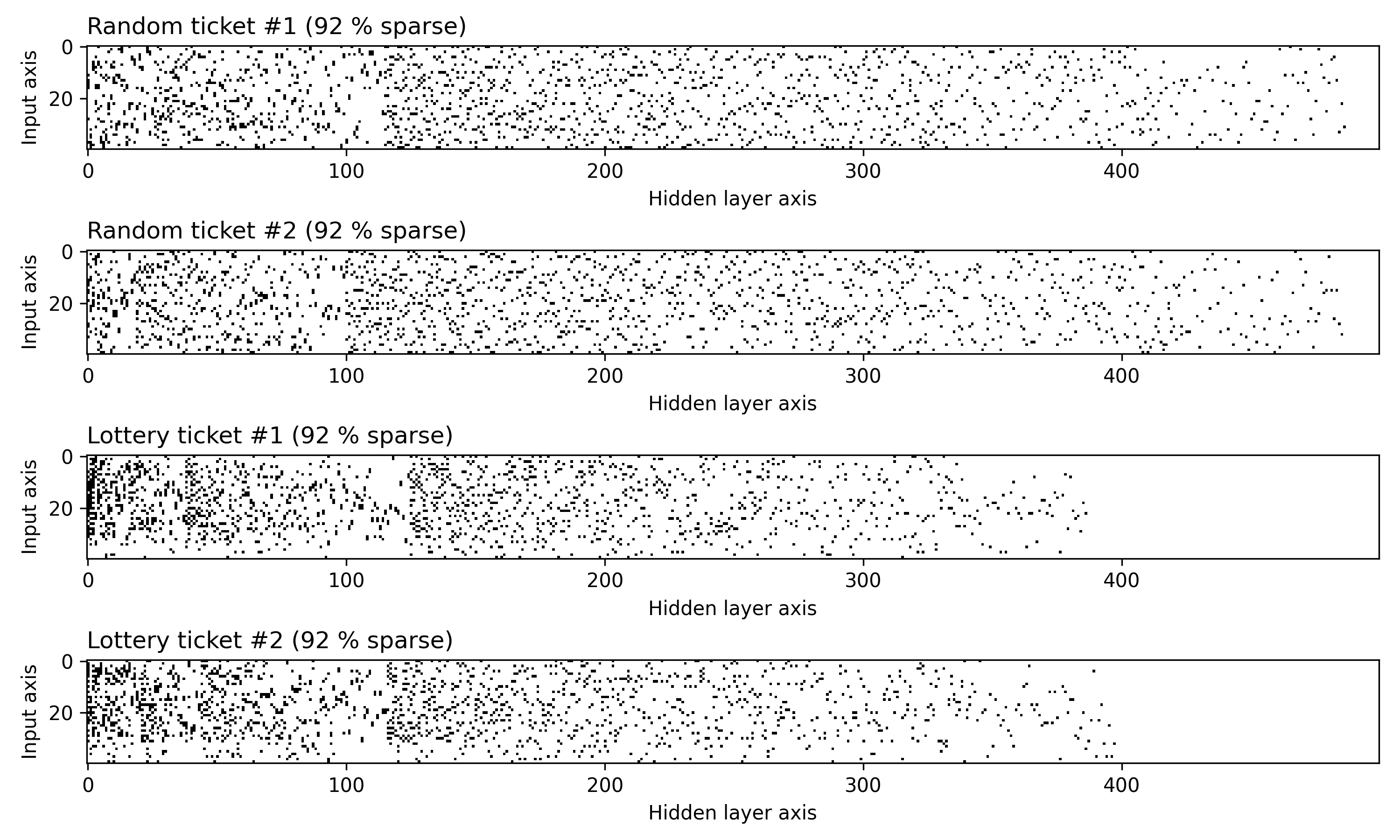
You can also visualize the actual masks selected via random and lottery pruning:
Visualize masks

Visualizing first layer weight masks of random tickets and lottery tickets. For interpretabilty, we have sorted the mask along the hidden layer axis according to the number of adjacent unmasked parameters. This helps reveal a bias towards local connectivity in the lottery ticket masks. Notice how there are many more vertically-adjacent unmasked parameters in the lottery ticket masks. These vertically-adjacent parameters correspond to local connectivity along the input dimension, which in turn biases the sparse model towards data with spatial structure. Best viewed with zoom.

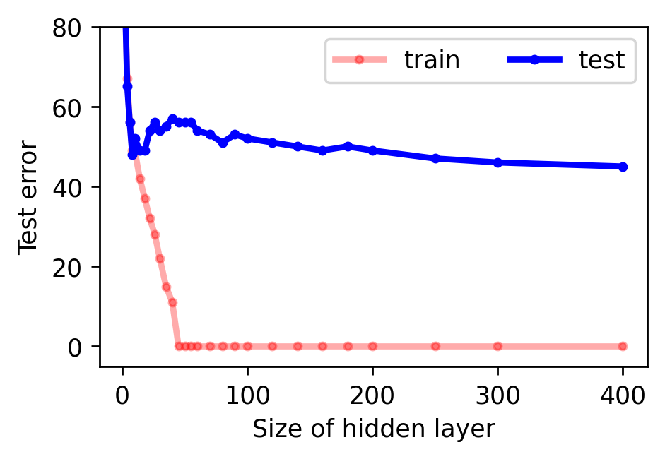
Observing deep double descent. Another intriguing property of neural networks is the “double descent” phenomenon. This phrase refers to a training regime where more data, model parameters, or gradient steps can actually reduce a model’s test accuracy^{1 2 3 4}. The intuition is that during supervised learning there is an interpolation threshold where the learning procedure, consisting of a model and an optimization algorithm, is just barely able to fit the entire training set. At this threshold there is effectively just one model that can fit the data and this model is very sensitive to label noise and model mis-specification.

Several properties of this effect, such as what factors affect its width and location, are not well understood in the context of deep models. We see the MNIST-1D dataset as a good tool for exploring these properties. In fact, we were able to reproduce the double descent pattern in a Colab notebook after just 25 minutes of walltime. The figure below shows our results for a fully-connected network. You can reproduce these results here.

Observing deep double descent. MNIST-1D is a good environment for determining how to locate the interpolation threshold of deep models.

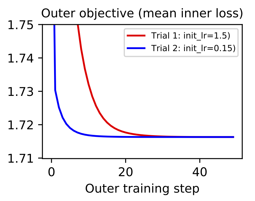
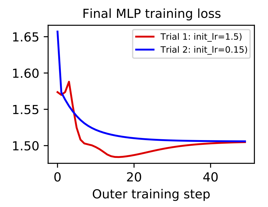
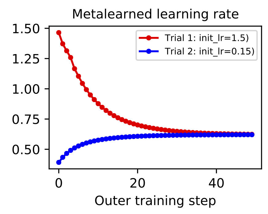
Gradient-based metalearning. The goal of metalearning is to “learn how to learn.” A model does this by having two levels of optimization: the first is a fast inner loop which corresponds to a traditional learning objective and second is a slow outer loop which updates the “meta” properties of the learning process. One of the simplest examples of metalearning is gradient-based hyperparameter optimization. The concept was was proposed by Bengio (2000) and then scaled to deep learning models by Maclaurin et al. (2015). The basic idea is to implement a fully-differentiable neural network training loop and then backpropagate through the entire process in order to optimize hyperparameters like learning rate and weight decay.

Metalearning is a promising topic but it is very difficult to scale. First of all, metalearning algorithms consume enormous amounts of time and compute. Second of all, implementations tend to grow complex since there are twice as many hyperparameters (one set for each level of optimization) and most deep learning frameworks are not set up well for metalearning. This places an especially high incentive on debugging and iterating metalearning algorithms on small-scale datasets such as MNIST-1D. For example, it took just a few hours to implement and debug the gradient-based hyperparameter optimization of a learning rate shown below. You can reproduce these results here.

Metalearning a learning rate: looking at the third plot, the optimal learning rate appears to be 0.6. Unlike many gradient-based metalearning implementations, ours takes seconds to run and occupies a few dozen lines of code. This allows researchers to iterate on novel ideas before scaling.

Metalearning an activation function. Having implemented a “minimal working example” of gradient-based metalearning, we realized that it permitted a simple and novel extension: metalearning an activation function. With a few more hours of researcher time, we were able to parameterize our classifier’s activation function with a second neural network and then learn the weights using meta-gradients. Shown below, our learned activation function substantially outperforms baseline nonlinearities such as ReLU, Elu⁵, and Swish⁶. You can reproduce these results here.

Metalearning an activation function. Starting from an ELU shape, we use gradient-based metalearning to find the optimal activation function of a neural network trained on the MNIST-1D dataset. The activation function itself is parameterized by a second (meta) neural network. Note that the ELU baseline (red) is obscured by the tanh baseline (blue) in the figure above.

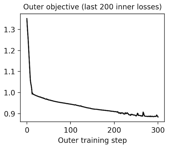
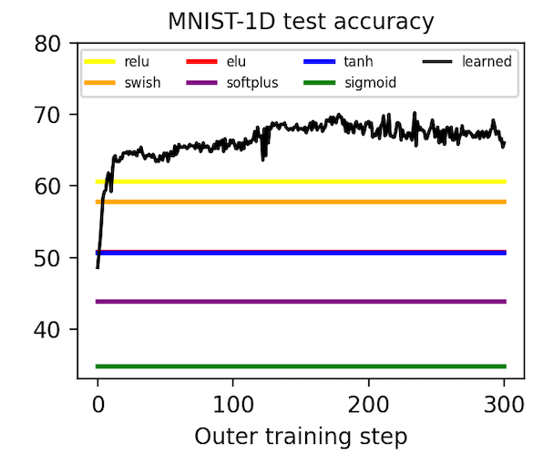
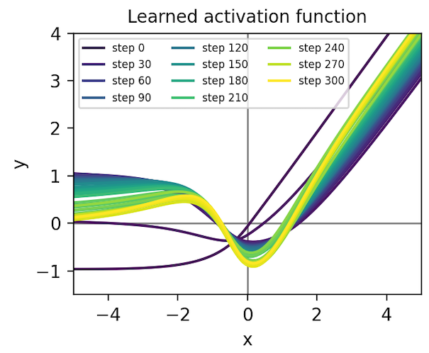
We transferred this activation function to convolutional models trained on MNIST and CIFAR-10 images and found that it achieves middle-of-the-pack performance. It is especially good at producing low training loss early in optimization, which is the objective that it was trained on in MNIST-1D. When we rank nonlinearities by final test loss, though, it achieves middle-of-the-pack performance. We suspect that running the same metalearning algorithm on larger models and datasets would further refine our activation function, allowing it to at least match the best hand-designed activation function. We leave this to future work, though.

Measuring the spatial priors of deep networks. A large part of deep learning’s success is rooted in “deep priors” which include hard-coded translation invariances (e.g., convolutional filters), clever architectural choices (e.g., self-attention layers), and well-conditioned optimization landscapes (e.g., batch normalization). Principle among these priors is the translation invariance of convolution. A primary motivation for this dataset was to construct a toy problem that could effectively quantify a model’s spatial priors. The second figure in this post illustrates that this is indeed possible with MNIST-1D. One could imagine that other models with more moderate spatial priors would sit somewhere along the continuum between the MLP and CNN benchmarks. Reproduce here.

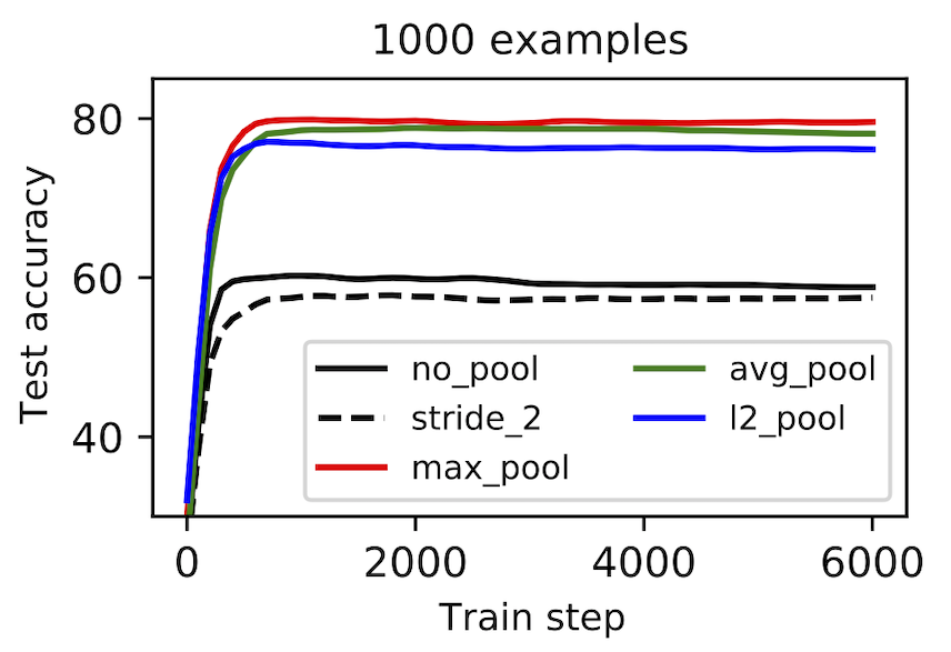
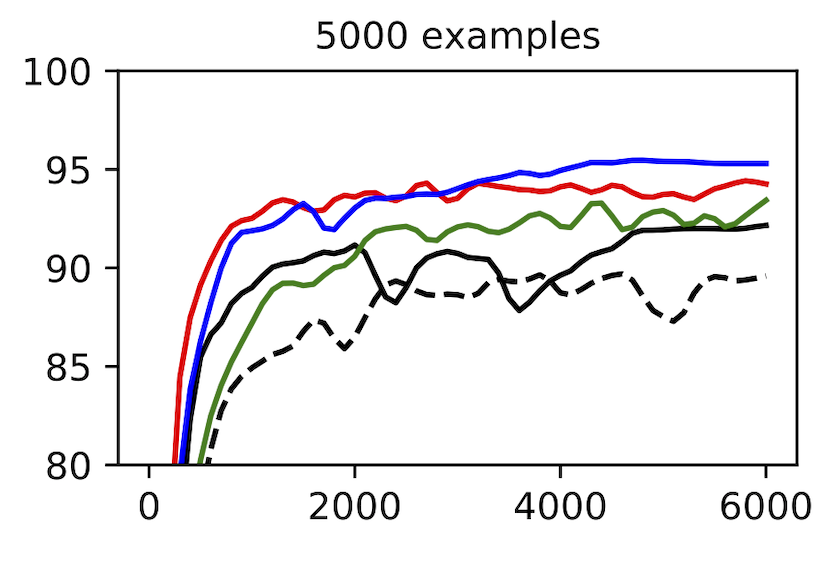
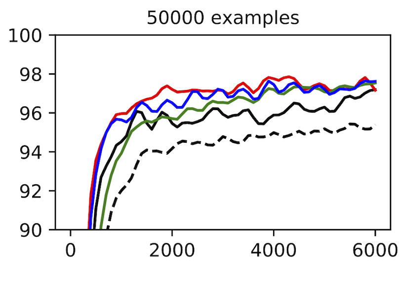
Benchmarking pooling methods. Our final case study begins with a specific question: What is the relationship between pooling and sample efficiency? We had not seen evidence that pooling makes models more or less sample efficient, but this seemed an important relationship to understand. With this in mind, we trained models with different pooling methods and training set sizes and found that, while pooling tended to be effective in low-data regimes, it did not make much of a difference in high-data regimes. We do not fully understand this effect, but hypothesize that pooling is a mediocre architectural prior which is better than nothing in low-data regimes and then ends up restricting model expression in high-data regimes. By the same token, max-pooling may also be a good architectural prior in the low-data regime, but start to delete information – and thus perform worse compared to L2 pooling – in the high-data regime. Reproduce here.

Benchmarking common pooling methods. We observe that pooling helps performance in low-data regimes and hinders it in high-data regimes. While we do not entirely understand this effect, we hypothesize that pooling is a mediocre architectural prior that is better than nothing in low-data regimes but becomes overly restrictive in high-data regimes.

When to scale

This post is not an argument against large-scale machine learning research. That sort of research has proven its worth time and again and has come to represent one of the most exciting aspects of the ML research ecosystem. Rather, this post argues in favor of small-scale machine learning research. Neural networks do not have problems with scaling or performance – but they do have problems with interpretability, reproducibility, and iteration speed. We see carefully-controlled, small-scale experiments as a great way to address these problems.

In fact, small-scale research is complimentary to large-scale research. As in biology, where fruit fly genetics helped guide the Human Genome Project, we believe that small-scale research should always have an eye on how to successfully scale. For example, several of the findings reported in this post are at the point where they should be investigated at scale. We would like to show that large scale lottery tickets also learn spatial inductive biases, and show evidence that they develop local connectivity. We would also like to try metalearning an activation function on a larger model in the hopes of finding an activation that will outperform ReLU and Swish in generality.

We should emphasize that we are only ready to scale these results now that we have isolated and understood them in a controlled setting. We believe that scaling a system is only a good idea once the relevant causal mechanisms have been isolated and understood.

Other small datasets

The core inspiration for this work stems from an admiration of and, we daresay, infatuation with the MNIST dataset. While it has some notable flaws – some of which we have addressed – it also has many lovable qualities and underappreciated strengths: it is simple, intuitive, and provides the perfect sandbox for exploring creative new ideas.

Our work also bears philosophical similarities to the Synthetic Petri Dish by Rawal et al. (2020). It was published concurrently and the authors make similar references to biology in order to motivate the use of small synthetic datasets for exploratory research. Their work differs from ours in that they use metalearning to obtain their datasets whereas we construct ours by hand. The purpose of the Synthetic Petri Dish is to accelerate neural architecture search whereas the purpose of our dataset is to accelerate “science of deep learning” questions.

There are many other small-scale datasets that are commonly used to investigate “science of deep learning” questions. The examples in the CIFAR-10 dataset are four times larger than MNIST examples but the total number of training examples is the same. CIFAR-10 does a better job of discriminating between MLP and CNN architectures, and between various CNN architectures such as vanilla CNNs versus ResNets. The FashionMNIST dataset is the same size as MNIST but a bit more difficult. One last option is Scikit-learn’s datasets: there are dozens of options, some synthetic and others real. But making real world analogies to, say, digit classification, is not possible and one can often do very well on them using simple linear or kernel-based methods.

Closing thoughts

There is a counterintuitive possibility that in order to explore the limits of how large we can scale neural networks, we may need to explore the limits of how small we can scale them first. Scaling models and datasets downward in a way that preserves the nuances of their behaviors at scale will allow researchers to iterate quickly on fundamental and creative ideas. This fast iteration cycle is the best way of obtaining insights about how to incorporate progressively more complex inductive biases into our models. We can then transfer these inductive biases across spatial scales in order to dramatically improve the sample efficiency and generalization properties of large-scale models. We see the humble MNIST-1D dataset as a first step in that direction.

Footnotes