Finding Paths of Least Action with Gradient Descent

Play

The purpose of this simple post is to bring to attention a view of physics which isn’t often communicated in introductory courses: the view of physics as optimization.

This approach begins with a quantity called the action. If you minimize the action, you can obtain a path of least action which represents the path a physical system will take through space and time. Generally speaking, physicists use analytic tools to do this minimization. In this post, we are going to attempt something different and slightly crazy: minimizing the action with gradient descent.

In this post. In order to communicate this technique as clearly and concretely as possible, we’re going to apply it to a simple toy problem: a free body in a gravitational field. Keep in mind, though, that it works just as well on larger and more complex systems such as an ideal gas – we will treat these sorts of systems in the paper and in future blog posts.

Now, to put our approach in the proper context, we’re going to quickly review the standard approaches to this kind of problem.

Standard approaches

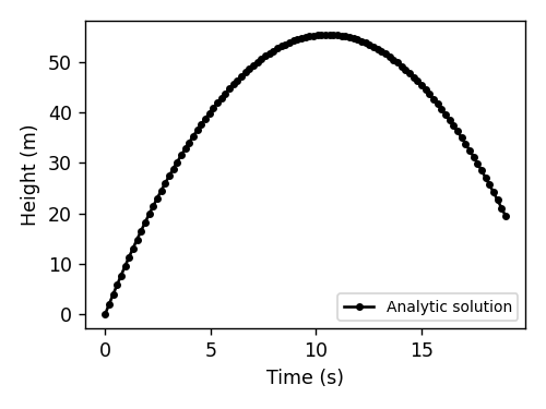
The analytical approach. Here you use algebra, calculus, and other mathematical tools to find a closed-form equation of motion for the system. It gives the state of the system as a function of time. For an object in free fall, the equation of motion would be:

def falling_object_analytical(x0, x1, dt, g=1, steps=100):
    v0 = (x1 - x0) / dt
    t = np.linspace(0, steps, steps+1) * dt
    x = -.5*g*t**2 + v0*t + x0  # the equation of motion
    return t, x

x0, x1 = [0, 2]
dt = 0.19
t_ana, x_ana = falling_object_analytical(x0, x1, dt)

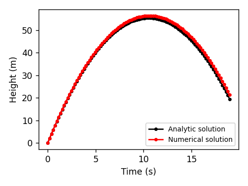
The numerical approach. Not all physics problems have an analytical solution. Some, like the double pendulum or the three-body problem, are deterministic but chaotic. In other words, their dynamics are predictable but we can’t know their state at some time in the future without simulating all the intervening states. These we can solve with numerical integration. For the body in a gravitational field, here’s what the numerical approach would look like:

def falling_object_numerical(x0, x1, dt, g=1, steps=100):
    xs = [x0, x1]
    ts = [0, dt]
    v = (x1 - x0) / dt
    x = xs[-1]
    for i in range(steps-1):
        v += -g*dt
        x += v*dt
        xs.append(x)
        ts.append(ts[-1]+dt)
    return np.asarray(ts), np.asarray(xs)

t_num, x_num = falling_object_numerical(x0, x1, dt)

Our approach: action minimization

The Lagrangian method. The approaches we just covered make intuitive sense. That’s why we teach them in introductory physics classes. But there is an entirely different way of looking at dynamics called the Lagrangian method. The Lagrangian method does a better job of describing reality because it can produce equations of motion for any physical system.¹ Lagrangians figure prominently in all four branches of physics: classical mechanics, electricity and magnetism, thermodynamics, and quantum mechanics. Without the Lagrangian method, physicists would have a hard time unifying these disparate fields. But with the Standard Model Lagrangian they can do precisely that.

How it works. The Lagrangian method begins by considering all the paths a physical system could take from an initial state \(\bf{x}\)\((t_0)\) to a final state \(\bf{x}\)\((t_1)\). Then it provides a simple rule for selecting the path \(\hat{\bf x}\) that nature will actually take: the action \(S\), defined in the equation below, must have a stationary value over this path. Here \(T\) and \(V\) are the kinetic and potential energy functions for the system at any given time \(t\) in \([t_0,t_1]\).

Finding \(\hat{\bf x}\) with Euler-Lagrange (what people usually do). When \(S\) is stationary, we can show that the Euler-Lagrange equation (third line in the equation above) holds true over the interval \([t_0,t_1]\) (Morin, 2008). This observation is valuable because it allows us to solve for \(\hat{\bf x}\): first we apply the Euler-Lagrange equation to the Lagrangian \(L\) and derive a system of partial differential equations.² Then we integrate those equations to obtain \(\hat{\bf x}\). Importantly, this approach works for all problems spanning classical mechanics, electrodynamics, thermodynamics, and relativity. It provides a coherent theoretical framework for studying classical physics as a whole.

Finding \(\hat{\bf x}\) with action minimization (what we are going to do). A more direct approach to finding \(\hat{\bf x}\) begins with the insight that paths of stationary action are almost always also paths of least action (Morin 2008). Thus, without much loss of generality, we can exchange the Euler-Lagrange equation for the simple minimization objective shown in the third line of the equation below. Meanwhile, as shown in the first line, we can redefine \(S\) as a discrete sum over \(N\) evenly-spaced time slices:

One problem remains: having discretized \( \hat{\bf{x}} \) we can no longer take its derivative to obtain an exact value for \( \dot{\bf{x}}(t_i) \). Instead, we must use the finite-differences approximation shown in the second line. Of course, this approximation will not be possible for the very last \( \dot{\bf{x}} \) in the sum because \(\dot{\bf{x}}_{N+1}\) does not exist. For this value we will assume that, for large \(N\), the change in velocity over the interval \( \Delta t \) is small and thus let \(\dot{\bf{x}}_N = \dot{\bf{x}}_{N-1}\). Having made this last approximation, we can now compute the gradient \(\frac{\partial S}{\partial \bf{x}}\) numerically and use it to minimize \(S\). This can be done with PyTorch (Paszke et al, 2019) or any other package that supports automatic differentiation.

A simple implementation

Let’s begin with a list of coordinates, x, which contains all the position coordinates of the system between t\(_1\) and t\(_2\). We can write the Lagrangian and the action of the system in terms of these coordinates.

def lagrangian_freebody(x, xdot, m=1, g=1):
    T = .5*m*xdot**2
    V = m*g*x
    return T, V
  
def action(x, dt):
    xdot = (x[1:] - x[:-1]) / dt
    xdot = torch.cat([xdot, xdot[-1:]], axis=0)
    T, V = lagrangian_freebody(x, xdot)
    return T.sum()-V.sum()

Now let’s look for a point of stationary action. Technically, this could be a minimum OR an inflection point.³ Here, we’re just going to look for a minimum:

def get_path_between(x, steps=1000, step_size=1e-1, dt=1, num_prints=15, num_stashes=80):
    t = np.linspace(0, len(x)-1, len(x)) * dt
    print_on = np.linspace(0,int(np.sqrt(steps)),num_prints).astype(np.int32)**2 # print more early on
    stash_on = np.linspace(0,int(np.sqrt(steps)),num_stashes).astype(np.int32)**2
    xs = []
    for i in range(steps):
        grad_x = torch.autograd.grad(action(x, dt), x)[0]
        grad_x[[0,-1]] *= 0  # fix first and last coordinates by zeroing their gradients
        x.data -= grad_x * step_size

        if i in print_on:
            print('step={:04d}, S={:.4e}'.format(i, action(x, dt).item()))
        if i in stash_on:
            xs.append(x.clone().data.numpy())
    return t, x, np.stack(xs)

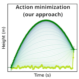
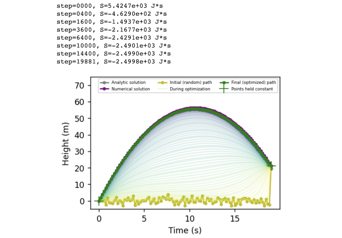
Now let’s put it all together. We can initialize our falling particle’s path to be any random path through space. In the code below, we choose a path where the particle bounces around x=0 at random until time t=19 seconds, at which point it leaps up to its final state of x = x_num[-1] = 21.3 meters. This path has a high action of S = 5425 J·s. As we run the optimization, this value decreases smoothly until we converge on a parabolic arc with an action of S = -2500 J·s.

dt = 0.19
x0 = 1.5*torch.randn(len(x_num), requires_grad=True)  # a random path through space
x0[0].data *= 0.0 ; x0[-1].data *= 0.0  # set first and last points to zero
x0[-1].data += x_num[-1]  # set last point to be the end height of the numerical solution

t, x, xs = get_path_between(x0.clone(), steps=20000, step_size=1e-2, dt=dt)

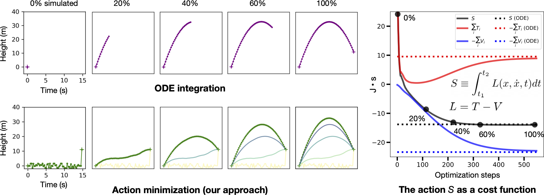
Direct comparison between the numerical (ODE) solution and our approach

On the left side of the figure below, we compare the normal approach of ODE integration to our approach of action minimization. As a reminder, the action is the sum, over every point in the path, of kinetic energy \(T\) minus potential energy \(V\). We compute the gradients of this quantity with respect to the path coordinates and then deform the initial path (yellow) into the path of least action (green). This path resolves to a parabola, matching the path obtained via ODE integration. On the right side of the figure, we plot the path’s action \(S\), kinetic energy \(T\), and potential energy \(V\) over the course of optimization. All three quantities asymptote at the respective values of the ODE trajectory.

Closing thoughts

As if by snake-charming magic, we have coaxed a path of random coordinates to make a serpentine transition into a structured and orderly parabolic shape – the shape of the one trajectory that a free body will take under the influence of a constant gravitational field. This is a simple example, but we have investigated it in detail because it is illustrative of the broader “principle of least action” which defies natural human intuition and sculpts the very structure of our physical universe.

By the vagueness of its name alone, “the action,” you may sense that it is not a well-understood phenomenon. In subsequent posts, we will explore how it works in more complex classical simulations and then, later, in the realm of quantum mechanics. And after that, we will talk about its history: how it was discovered and what its discoverers thought when they found it. And most importantly, we will address the lingering speculations as to what, exactly, it means.

Footnotes