Pointer Theory

This post is about how simulating the universe could give rise to quantum mechanics. My first attempt at this topic, written a few years ago, is here. You can also read this article as a Colab notebook.

Quantum mechanics makes powerful predictions about the world, but the theory itself is hard to wrap one’s mind around. This is not just because it comes with a lot of complex mathematical machinery, but also because it violates some core axioms of physics that are sacred everywhere else.

First, it breaks local realism, which is actually a pair of constraints that say “things cannot be two things at once” and “things can only interact with their immediate neighbors”. It breaks both of these: regarding realism, it says that states exist in superpositions; regarding locality, it says that wavefunction collapse happens instantaneously across space and time.

Second, it permits large-scale entangled systems, such as a mole of entangled atoms, which require much more information/compute than exists in the entire universe to compute/evolve. These are deep problems with quantum mechanics, and I have always felt that something about the core thought experiment must be wrong.¹

What we might prefer is an thought experiment that reveals quantum phenomena to be elegant and even perhaps inevitable properties of the universe. Finding such an thought experiment is the purpose of this post.

Deriving Pointer Theory

First, imagine that the universe is being simulated. It’s helpful to do this even if you don’t think that it is actually how the world works, because physics simulations have the same forcing functions as reality. To see this clearly, consider the Minimum Description Length (MDL) principle. It says that, for a given dataset, the model that gives the most concise description of the data is best. This principle, applied to our observations of the universe, says that the physics simulator which is most true to reality is the one that reproduces what we know about the universe using the least amount of code and computation.²

Practically speaking, here are three constraints that, at a minimum, the architect of a very large-scale simulation would want to prioritize:

1. Massive parallelism. Taking advantage of the fact that, in physics, most (all?) interactions are local and limited by the speed of light, one could parallelize the simulation. Spatially adjacent regions would run on the same devices whereas spatially distant regions would run on separate ones (by devices we mean CPUs, GPUs, etc)
2. Conservation laws enforced. Physics is built on the idea that certain quantities are strictly conserved. Scalar quantities like energy are conserved, as are vector quantities like angular momentum.
3. Isotropy. Space must be uniform in all directions; physics has to be invariant under rotation.

The first thing to see is that assumptions 1 and 2 are in tension with one another. In order to ensure that a quantity like energy is conserved, you need to sum that quantity across the entire simulation, determine whether a correction is needed, and then apply that correction to the system as a whole. Computationally, this normalization step requires a synchronous reduction operation and an element-wise divide at every timestep.

When you write a single-threaded physics simulation, this can account for about half of the computational cost. As you parallelize your simulation more and more, you can expect the cost of enforcing conservation laws with a naive global operation to grow higher in proportion until they dominate. This is because simulating local interactions is pretty easy to do in parallel, but enforcing system-wide conservation laws requires transferring data between distant chips and keeping them more or less in sync. As a result, enforcing conservation laws quickly grows to be a limiting factor.

We find ourselves asking if there is a more parallelizable approach.

It turns out that there are several more parallelizable approaches, but I was only able to find one³ with numerical exactness (don’t drift when simulating extremely long time horizons and very high-energy, high-curvature physics) and strong parallelism (no global operations permitted, ever):

Scalar conservation laws (e.g. energy) are easy: discretize them. If you want a mental model, think of how finance treats money as continuous but makes pennies the indivisible floor to keep rounding errors from accumulating. Each region can spend and receive whole quanta without ever consulting a global ledger. We’ll call this approach “discrete local flux enforcement.”

Vector conservation laws (e.g. angular momentum) are harder. You can’t just discretize angles because picking a finite set of allowed directions breaks rotational symmetry (see assumption #3). But we can try a different trick: when two particles share a conserved vector, you store a nonlocal hidden variable - an array of amplitudes over the joint measurement outcomes — and give both particles a pointer to it. Measurement overwrites the shared variable and every reference feels the update instantly⁴. Since this approach to enforcing vector conservation laws rests on giving particles pointers to a shared nonlocal variable, we call it pointer theory.

Discrete local flux enforcement can conserve scalars exactly, but when a vector conservation law has to hold between two spacelike-separated measurements, local enforcement provably cannot coordinate the joint outcome. This is actually the conclusion of Bell’s theorem. And so you have to violate locality if you want to conserve vector quantities (while preserving realism). Pointer theory, or something similarly nonlocal, is the inevitable solution.⁵

Comparison to Quantum Mechanics

Pointer theory is similar to quantum mechanics in the sense that both can be used to explain the empirical behavior of fundamental particles at quantum scale. However, the two theories give very different explanations for how reality works. The key area where they diverge is in their interpretation of the Bell theorem. The Bell theorem says that in order to explain certain experimental results, you must give up realism (the idea that particles have definite state) or locality (the idea that particles only influence their neighbors). Because of this result, quantum mechanics has chosen to sacrifice realism in order to preserve locality. Meanwhile, by way of a nonlocal hidden variable, pointer theory sacrifices locality in order to preserve realism.⁶

Quantum mechanics says that subatomic particles occupy all possible states before observation, the wavefunction can collapse instantaneously across space according to no known mechanism, and entangled systems can grow exponentially without bound. Pointer theory, by taking the realist fork of the Bell inequality, leads to a somewhat more concrete setup, the kind of setup one can implement cleanly in code. In the pointer theory setup, the wavefunction is a concrete array of numbers shared between entangled particles. Entanglement, then, is just shared mutable state and wavefunction collapse is what happens when we edit that shared state to remove the thing that was just measured. Measurement is an overwrite to part of the shared underlying state of a set of particles.

Implications

This theory is hard to test because it gives mostly the same predictions as quantum mechanics. The only place where it may diverge is in cases where the entanglement of the system is very high. This is the exact regime that quantum computing efforts are currently probing, because high entanglement (high Schmidt rank) yields high numbers of effective qubits.

I was interested to find that no known natural phenomena have effective entanglements as high or stable as what has been achieved artificially in quantum computers. Most entanglement structures in nature are extremely low dimensional and very short-lived. Entanglement structures are constantly breaking and re-forming; this means that they can affect the behavior of molecules to a high degree, but they are actually often much lower-dimensional and more short-lived than even how we represent them when we run simulations of those molecules.

At any rate, the reason this discussion of high-entanglement regimes is important is that the amount of memory and compute needed to represent an entangled state grows exponentially in relation to the number of effective qubits. And so, for relatively small numbers of effective qubits (eg, only 100-300) the amount of memory needed by the simulation we have hypothesized, just to represent them, would begin to approach the size of the entire rest of the simulation. And so, if we assume that the shared state that holds entanglement in the simulation has limited memory and compute, then we should expect it to have a hard cap on the total number of effective qubits allowed.

This could manifest as a “soft cap” where at some point it gets exponentially harder for us to add additional qubits to quantum computers, or it could (though arguably less likely) manifest as a plateau or regime change. The mechanism here might be similar to what state-of-the-art classical quantum simulation techniques like MPS and PEPS do: they set a maximum “bond dimension” beyond which additional entanglement is not allowed, and then for any entanglement above that ceiling they approximate it as best they can.

The idea that nature itself may have a ceiling on the number of qubits we can build may sound like a dramatic prediction, but consider the alternative: if there were no maximum bond dimension, then it should, in principle, be possible to entangle an entire mole of atoms. Just evolving the wavefunction for this system would require much more information than exists in the entire universe! And even if the wavefunction is not a “real” object (and this not subject to information limits, as some physicists argue), the computation required to evolve a state with \(6×10^{23}\) atoms would still have to be done somewhere, and that work, \(\approx 10^{(1.8×10^{23})}\) operations for even a single timestep, exceeds the computational history of the observable universe (\(\approx 10^{120}\) operations) by a large margin.

It is possible that nature really does have a maximum bond dimension for highly entangled systems. If this were the case, it would close the loop on the argument that began this post: we derived the theory by assuming a simulator with a finite memory and compute budget, and a cap on bond dimension is what that budget looks like from inside the simulation. Established quantum theory does not provide an equivalent mechanism.

Code examples

Let’s walk through a few simple code examples to intuit how pointer theory would work in practice. Warning: it will look similar to quantum mechanics, but there are differences in notation and style. The first example we’ll consider is the most important experiment for us - the CHSH experiment which is the basis for Bell’s theorem, and which in turn is the most fundamental claim of quantum mechanics.

The CHSH Bell Inequality

The Bell inequality says that in order to explain certain experimental results, you must give up realism (the idea that particles have definite state) or locality (the idea that particles only influence their neighbors). Quantum mechanics solves this by giving up realism, and because the results of this way of thinking are well documented on Wikipedia and most quantum courses, we will say no more. Our purpose here is to show that pointer theory, which chooses to give up locality and preserve realism, is an equally viable option. With that in mind, let us describe and then simulate the experimental setup used by CHSH, first using a local hidden variable model (a local shared state; also referred to as a classical solution) and then using pointer theory.

Setup. A source emits two entangled photons. Alice and Bob each pick a polarizer angle and record ±1. The CHSH statistic \(|S|\) is bounded by 2 for any local hidden-variable theory; real life versions of this experiment measure \(|S|\) at \(2 \sqrt 2 \approx 2.83\), and so this is the number that we need to recover. Pointer theory, with an in-place shared state overwrite, allows us to reproduce this number.

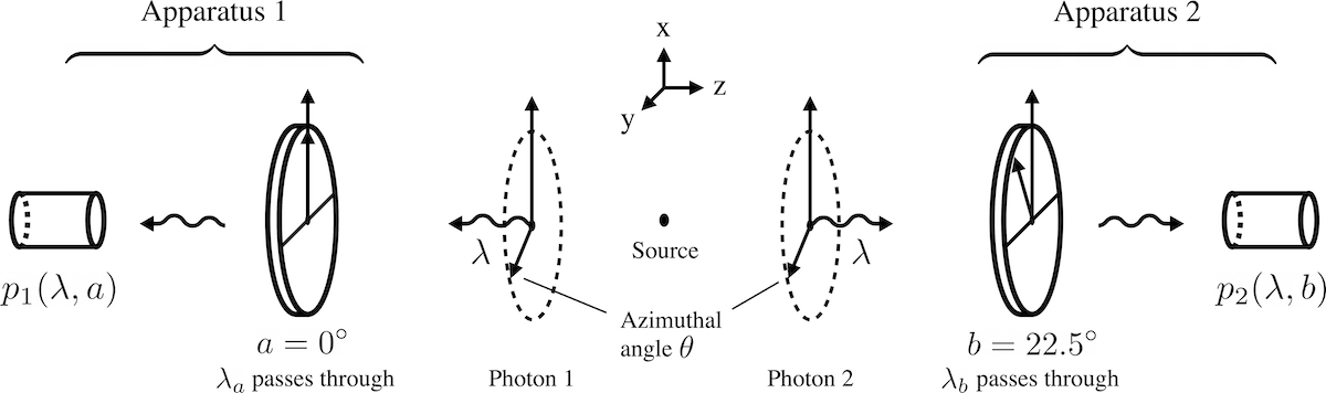
a, b = 0.0, math.pi / 8  # polarizer settings (Apparatus 1, Apparatus 2 in the figure)

def measure(state, angle):                          # sample ±1 from the shared scalar
    return +1 if np.random.random() < math.cos(state - angle) ** 2 else -1

def trial_local(a, b):                              # shared_state is read but never written
    state = np.random.uniform(0, 2 * math.pi)
    return measure(state, a) * measure(state, b)

def trial_nonlocal(a, b):
    state = np.random.uniform(0, 2 * math.pi)
    o1 = measure(state, a)
    state = a + math.pi / 2 if o1 == +1 else a      # <-- THE WHOLE MECHANISM 
    return o1 * measure(state, b)

print(f'local state:    average(o1·o2) = {np.mean([trial_local(a, b) for _ in range(10_000)]):+.3f}')
print(f'nonlocal state: average(o1·o2) = {np.mean([trial_nonlocal(a, b) for _ in range(10_000)]):+.3f}   (QM: {-math.cos(2*(a-b)):+.3f})')

Output:

local state:    average(o1·o2) = +0.336
nonlocal state: average(o1·o2) = -0.701   (QM: -0.707)

def chsh(trial, n=50_000):                # S = |E(a1,b1) - E(a1,b2) + E(a2,b1) + E(a2,b2)|
    a1, a2 = 0.0, math.pi / 4             # Alice's two polarizer settings
    b1, b2 = math.pi / 8, 3 * math.pi / 8 # Bob's, 22.5° off Alice's (for maximum violation)
    E = lambda a, b: np.mean([trial(a, b) for _ in range(n)])
    return abs(E(a1, b1) - E(a1, b2) + E(a2, b1) + E(a2, b2))

print(f'local state:    |S| = {chsh(trial_local):.3f}   (LHV bound: |S| ≤ 2)')
print(f'nonlocal state: |S| = {chsh(trial_nonlocal):.3f}   (QM: |S| = 2√2 ≈ {2*math.sqrt(2):.3f})')

Output:

local state:    |S| = 1.419   (LHV bound: |S| ≤ 2)
nonlocal state: |S| = 2.831   (QM: |S| = 2√2 ≈ 2.828)

Pointing to an array instead of a scalar

Simulating three entangled particles is harder than two and requires that we represent shared_state as an array instead of a scalar. This is because an equatorial Bell pair (fully entangled, single measurement plane) conserves angular momentum via perfect anticorrelation, whereas with three particles (or partial entanglement) we need to do a bit more bookkeeping.

In a state with, say, three particles, Alice’s measurement fixes one term in the conservation law, but what’s left is a constraint between the two unmeasured particles. A scalar \(\lambda\) has nowhere to put such a pair-relationship and so, to make things work, we need to use an N-dimensional complex array, then collapse it along the measured axis, and then maintain entanglement everywhere else. We accomplish this with a single function called project, which - as its name suggests - projects out the entanglement associated with the measured particle.

Specific notes. In the code above, you will see that we used the GHZ state, which is a 3-particle shared state represented as \((|000\rangle + |111\rangle)/\sqrt 2\). The shared state is a 2×2×2 array with equal amplitude on the all-zeros and all-ones outcomes. \(M\) defined as \(\langle XXX\rangle - \langle XYY\rangle - \langle YXY\rangle - \langle YYX\rangle\) (Mermin, 1990) has an LHV (local hidden variable theory) bound of \(|M|\le 2\) but experiment has shown that it is exactly 4. Pointer theory and quantum mechanics both yield a value of 4.

X = np.array([[0, 1], [1, 0]], complex)
Y = np.array([[0, -1j], [1j, 0]], complex)
Z = np.array([[1, 0], [0, -1]], complex)

def axis_op(basis):                                                    # scalar angle (X-Y plane) or (theta, phi) tuple (sphere)
    if isinstance(basis, tuple):
        theta, phi = basis
        return np.sin(theta)*np.cos(phi)*X + np.sin(theta)*np.sin(phi)*Y + np.cos(theta)*Z
    return np.cos(basis)*X + np.sin(basis)*Y

def project(shared_state, which_particle, basis=None):
    """Measure `which_particle` of the joint state (a complex array, one axis per particle). `basis`
    is a scalar angle (X-Y plane), (theta, phi) tuple (sphere), or None (standard basis).
    Born-samples an outcome, zeros the inconsistent slices, returns (collapsed_state, ±1 or index)."""
    shared_state = np.moveaxis(shared_state, which_particle, 0)     # bring measured particle to front
    if basis is not None:                                           # rotate into measurement basis
        _, V = np.linalg.eigh(axis_op(basis))                       # columns of V are outcome states
        shared_state = np.tensordot(V.conj().T, shared_state, axes=1)

    # rows = outcomes; columns = other particle states
    flat = shared_state.reshape(shared_state.shape[0], -1)

    # Born rule: P(outcome) = sum |amplitude|^2 over rest
    probs = (np.abs(flat) ** 2).sum(axis=1)
    outcome = np.random.choice(len(probs), p=probs / probs.sum())

    # collapse: keep only the slice consistent with outcome
    new = np.zeros_like(shared_state); new[outcome] = shared_state[outcome]
    if basis is not None: new = np.tensordot(V, new, axes=1)        # rotate back to original basis
    new = np.moveaxis(new, 0, which_particle) / np.linalg.norm(new)

    # position returns cell index; spin returns ±1
    label = outcome if basis is None else (-1, +1)[outcome]
    return new, label


#### Show off this new code on a simulation of the 3-particle GHZ state ####

def ghz_state():
    p = np.zeros((2, 2, 2), complex); p[0, 0, 0] = p[1, 1, 1] = 1/np.sqrt(2); return p

def correlator3(axes, n_trials):                     # <a·b·c> at one triple of measurement angles
    total = 0
    for _ in range(n_trials):
        shared_state, prod = ghz_state(), 1
        for i, ax in enumerate(axes):
            shared_state, o = project(shared_state, i, ax); prod *= o
        total += prod
    return total / n_trials

def mermin_M(n_trials=300):
    Xa, Ya = 0.0, np.pi / 2                          # X-axis and Y-axis angles in the X-Y plane
    return abs(correlator3((Xa, Xa, Xa), n_trials)
             - correlator3((Xa, Ya, Ya), n_trials)
             - correlator3((Ya, Xa, Ya), n_trials)
             - correlator3((Ya, Ya, Xa), n_trials))

print(f'pointer theory   |M| = {mermin_M():.3f}')
print(f'LHV bound        |M| ≤ 2.000')
print(f'QM               |M| = 4.000')

Output:

pointer theory   |M| = 4.000
LHV bound        |M| ≤ 2.000
QM               |M| = 4.000

Closing thoughts

This post introduces pointer theory, an alternative explanation for what is going on in quantum mechanics. It is based on a thought experiment where we assume the universe is simulated and subject to 1) massive parallelization 2) strictly enforced conservation laws, and 3) a limited compute/memory budget. Pointer theory predicts known experimental phenomena accurately (it looks just like quantum mechanics in most regimes) but for very high numbers of effective qubits it preducts we may eventually find a soft ceiling.

I think that this soft ceiling prediction (which, by the way, one or two other fringe theories have as well) is one of the more interesting results, as it saves us from the theoretical problems associated with allowing entanglement to scale indefinitely.

Footnotes