A Bird's Eye View of Synthetic Gradients

Synthetic gradients in action (from the DeepMind blog post)

Synthetic gradients achieve the perfect balance of crazy and brilliant. In a 100-line Gist I’ll introduce this exotic technique and use it to train a neural network.

Some Theory

Backprop (gradient backpropagation) is a way to optimize neural networks. As a quick review, there are two important functions for training a neural network:

1. the feedforward function
   • \[\hat y_i = f(x_i,\theta)\]
2. the loss function (I’ll use L2 loss)
   • \[L = \sum_i \frac{1}{2}(y_i-\hat y_i)^2\]

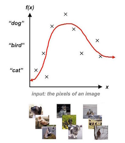
In supervised learning, the objective is to make the feedforward function approximate the true mapping from the input data \(x_i\) to the target label \(y_i\). The input \(x_i\) could be the pixels of an image and \(y_i\) could be a label for that image. Or, \(x_i\) could be a sentence in French and \(y_i\) could be a sentence in English. The mapping could really be any function! The loss measures how well the neural network learns to approximate this mapping.

Deep learning as a type of regression (images from 2015 ImageNet paper)

We can minimize the loss by adjusting each of the network’s parameters \(\theta_i\) just slightly. In order to do this, we compute the gradient of the loss function with respect to \(\theta_i\), multiply by a small number \(\alpha\) (the learning rate), and add this to the current value of \(\theta_i\).

Hopefully this is all review. If not, check out Stanford’s CS231n course notes or my very own math+code derivation of backprop.

Theory. From a theory perspective, backprop is easy to derive and works perfectly as long as the feedforward function is differentiable. Better yet, for small enough \(\alpha\), gradient descent with backprop is guaranteed to converge. In fact, it will probably converge to a global minimum.

Autodifferentiation. If we break the feedforward function of a neural network into its component functions, we can represent it as a directed graph where each junction is an operation and data flows along the vertices. The graph of a two-layer neural network with sigmoid activations might look like this:

Forward pass

We would implement this network in a numpy one-liner such as

y_hat = sigmoid(np.dot(sigmoid(np.dot(x, W1) + b1), W2) + b2)

During backprop, we recursively apply the chain rule to the feedforward function. Each recursive step moves the gradient backwards through one of the functions in the graph above. This means we can represent backprop using the same sort of graph:

Backward pass

See how we can map each node in the forward pass to a node in the backward pass. In other words, if we know the forward pass, we can automatically compute the backward pass. This is called autodifferentiation and all modern deep learning libraries (Theano, TensorFlow, Torch, etc.) can do it. The user simply builds a computational graph of the forward pass and the software handles the backwards pass. Pretty slick!

Full pass with mapping between forward and backward passes

Locking. When we train deep models with backprop, we must evaluate the entire forward pass before computing the backward pass. Worse still, each node in the forward and backward passes must be evaluated in the order that it appears. All nodes of the graph are effectively ‘locked’ in the sense that they must wait for the remainder of the network to execute forwards and propagate error backwards before a second update.

In practice, this causes trouble for

1. recurrent models (backprop through time makes the graph very deep)
2. training models in parallel (asynchronous cores must wait for one another)
3. models with different timescales (some layers must update more often than others)

Unlocking. The paper that inspired this blog post is Decoupled Neural Interfaces using Synthetic Gradients. DeepMind researchers propose an ambitious method for ‘unlocking’ neural networks: train a second model to predict the gradients of the first. In other words, approximate

When I realized what they were trying to do, I rolled my eyes. You must need to know more about the model to approximate its gradients…a model to predict the gradients wouldn’t train quickly enough…even if it did, backprop would still converge more quickly…

It turns out that simple linear regression can effectively map a layer’s activations to its gradients. More than that, it gives good results. I was so stunned (and frankly suspicious) that I set out to prove it.

Let’s prove it!

MNIST training samples

The data. Just as in my regularization post, we’ll train our model on the MNIST classification task. I chose the MNIST dataset because it’s easy to interpret, reasonably complex, and TensorFlow has a great MNIST utility.

Implementing regular backprop. In a regular training loop, we load the data, send it through the feedforward function, and calculate the loss. Next we use y_hat (the model’s prediction) and y (the training labels) to calculate gradients and perform a gradient update. Check out the pseudocode for this process below.

for i in xrange(train_steps):
    X, y = mnist.train.next_batch(batch_size) # load data
    
    y_hat, hs = forward(X, model) # forward pass on MNIST model
    
    # compute the average cross-entropy loss
    y_logprobs = -np.log(y_hat[range(batch_size),y]) # we want probs on the y labels to be large
    loss = np.sum(y_logprobs)/batch_size + reg_loss

    grads = backward(y, y_hat, hs, model) # data gradients
    model = {k : model[k] - learning_rate*grads[k] for (k,v) in grads.iteritems()} # update model

Implementing synthetic gradients. The training loop for synthetic gradients is a little different. We load data and perform the forward pass as usual. Next, we compute the gradients by sending the activations from the MNIST model (model) through a second model (smodel). For every ten parameter updates of the MNIST model we perform a parameter update on smodel. The smodel updates, contained inside the if statement, use regular backprop.

for i in xrange(train_steps):
    X, y = mnist.train.next_batch(batch_size) # load data
    
    y_hat, hs = forward(X, model) # forward pass on MNIST model
    synthetic_grads = sforward(hs, smodel, model) # forward pass on synthetic gradient model

    # update synthetic gradient model (smodel)
    if i % 10 == 0:
        # compute the MNIST model's loss and gradients...
        # compute smodel's loss and gradients (sgrads)...
        # update smodel parameters
        smodel = {k : smodel[k] - slearning_rate*sgrads[k] for (k,v) in sgrads.iteritems()}
    
    # reshape the synthetic gradients...
    # update the MNIST model with synthetic gradients
    model = {k : model[k] - learning_rate*v for (k,v) in synthetic_grads.iteritems()}

Pros and Cons

Stale gradients. Let’s compare our ‘unlocked’ MNIST model to one trained with backprop using stale gradients. To train with stale gradients, compute the gradient with backprop once every ten steps and otherwise use it to perform a parameter update. Since we use the same gradient for multiple parameter updates, we call it ‘stale.’ Using stale gradients is a good way to compare synthetic gradients to regular gradients because both perform backprop at the same rate (just once every ten training steps).

Stale vs. synthetic gradients. Final accuracies were 90.0% and 89.9% respectively

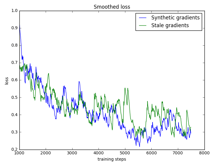
As we would expect for a small model, stale and synthetic gradients are evenly matched. The plot shows that the two methods converge at roughly the same rate. For wider, deeper models and more complicated versions of smodel, synthetic gradients can easily outperform stale ones. Mild pro.

Visualizing the difference. A more qualitative way to compare synthetic and actual gradients is to stop the training loop at a random time step and plot heatmaps of the two, side by side.

Visualizing gradients at the second layer of a 2-layer MNIST classifier.

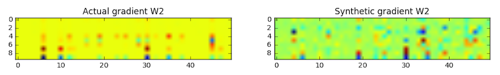
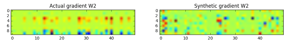
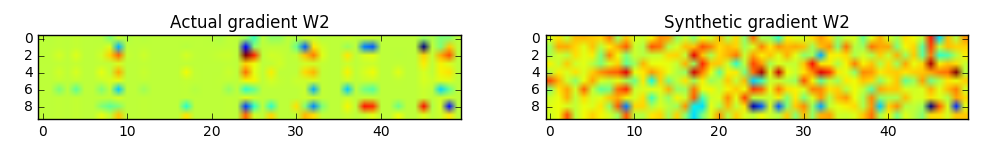
There is a definite correspondence between actual and synthetic gradients, particularly for the darker points. Even though the synthetic model makes mistakes, it seems to be making a good overall approximation. Medium pro.

Runtime.

EDIT: I made a mistake in my implementation of synthetic gradients. Runtime is not the issue I imagined it was because the targets of the synthetic gradient models should be the output activations of each layer rather than the actual gradients on the weights. I’m in the process of fixing this in my code. For now, ignore this portion of the post.

The DeepMind paper was mysteriously quiet about runtime. Why? Because it’s horrific! For my toy model, normal backprop is 100-1000x faster. Why? Well, let’s count parameters.

Consider two adjacent, fully connected layers \(l_I\) and \(l_J\) with \(m\) and \(n\) hidden units respectively. Now construct a simple linear regression model that maps the activation \(h_J\) to \(\nabla \theta_J\) (the approximate gradient of all parameters in \(l_J\)). The dimensionality of the input is \(n\) and that of the target is \((m+1) \times n\). Our simple linear model will have a total of \(n^2(m+1)(n+1) \approx O(mn^3)\) parameters. This means that synthetic gradient model will be larger and more expensive to train than the original model by a factor of \(O(n^2)\). Strong con!

Much to my surprise, synthetic gradients were able to approximate actual gradients and train a model to classify MNSIT digits. The large number of additional parameters required to make this happen, though, might be a dealbreaker.

Let’s review. Much to my surprise, synthetic gradients were able to approximate actual gradients and train a model to classify MNIST digits. The large number of additional parameters required to make this happen, though, might be a dealbreaker. Before synthetic gradients become a practical tool, researchers must find a way to reduce the number of regression parameters. In the meantime, backprop will remain supreme.

Puppy or Bagel?

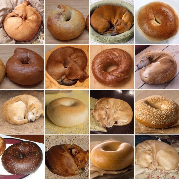
Imagine you’re a researcher tossing around the idea of synthetic gradients. How could you tell whether it’s a crazy idea that will waste your time or a useful idea that will make a difference? It’s a tricky question…a little like the infamous puppy vs. bagel meme.

Puppy or bagel?

This may sound cheesy, but the trick is to eat a lot of bagels and pet a lot of puppies :). In other words, finding good research ideas means exploring the crazy ones first. I really mean exploring. This term I spent two weeks exploring an adversarial LSTM idea that failed horribly. That said, it taught me what I - and the deep learning algorithm I used - can and can’t do.

Another example. Science is full of crazy ideas that end up working. Take quantum mechanics and the theory of electron spin. It started in 1925 when two physics grad students (George Uhlenbeck and Samuel Goudsmit) realized that treating an electron as if it were a spinning sphere helped with their calculations. There was only one problem: the electron would need to be spinning faster than the speed of light. Even though this was clearly impossible, their advisor, Paul Ehrenfest, called it a “very witty idea” and the theory of electron spin was born.

Synthetic gradients sound like a crazy idea right now, but maybe future innovations will shape them into a practical tool. They could become a key method for, say, training deep learning models on thousands of machines at once. Since asynchonicity matters as much as runtime efficiency on large computing clusters, this is not unrealistic.

Takeaway. I was surprised that synthetic gradients were so easy to implement. In fact, any enthusiastic undergraduate with CS skills (like myself) could have come up with the original idea. It’s encouraging to think that other ideas - just as crazy and brilliant - are still out there, hidden in plain sight.