
Lagrangian Neural Networks
Accurate models of the world are built on notions of its underlying symmetries. In physics, these symmetries correspond to conservation laws, such as for energy and momentum. But neural network models struggle to learn these symmetries. To address this shortcoming, last year I introduced a class of models called Hamiltonian Neural Networks (HNNs) that can learn these invariant quantities directly from (pixel) data. In this project, some friends and I are going to introduce a complimentary class of models called Lagrangian Neural Networks (LNNs). These models are able to learn Lagrangian functions straight from data. They’re interesting because, like HNNs, they can learn exact conservation laws, but unlike HNNs they don’t require canonical coordinates.
“A scientific poem”
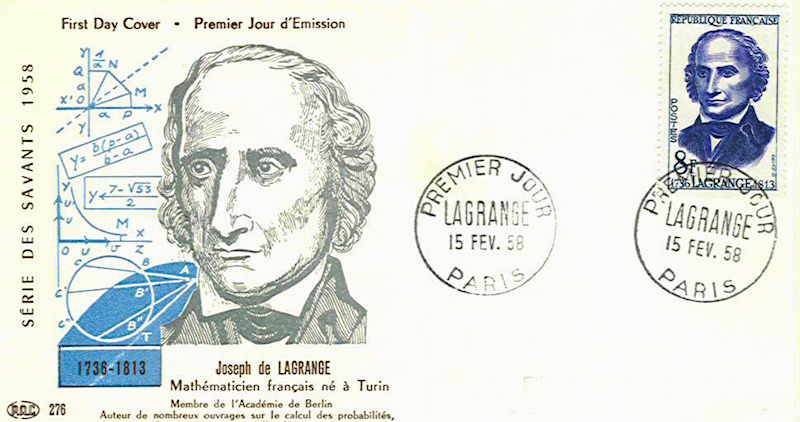
Joseph-Louis Lagrange must have known that life is short. He was born to a family of 11 children and only two of them survived to adulthood. Then he spent his adult years in Paris, living through the Reign of Terror and losing some of his closest friends to the guillotine. Sometimes I wonder if these hardships made him more sensitive to the world’s ephemeral beauty, and more determined to make the most of his short time here.
Indeed, his path into research was notable for its passion and suddenness. Until the age of 17, Lagrange was a normal youth who planned to become a lawyer and showed no particular interest in mathematics. But all of that changed when he read an inspiring memoir by Edmund Halley and decided to embark on an obsessive course of self-study in mathematics. A mere two years later he published the principle of least action.
“I will deduce the complete mechanics of solid and fluid bodies using the principle of least action.” – Joseph-Louis Lagrange, age 20
Lagrange’s work was notable for its purity and beauty, especially in contrast to the chaotic and broken times that he lived through. Expressing admiration for the principle of least action, William Hamilton once called it “a scientific poem”. In the following sections, I’ll introduce you to this “scientific poem” and then use it to derive Lagrangian Neural Networks.
The Principle of Least Action
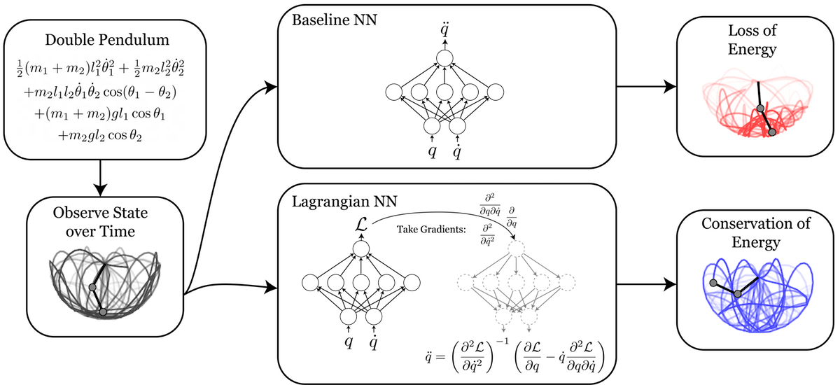
The Action. Start with any physical system that has coordinates \(x_t = (q, \dot q)\). For example, we might describe a double pendulum using the angles of its arms and their respective angular velocities. Now, one simple observation is that these coordinates must start in one state \(x_0\) and end up in another, \(x_1\). There are many paths that these coordinates might take as they pass from \(x_0\) to \(x_1\), and we can associate each of these paths with a scalar value \(S\) called “the action.” Lagrangian mechanics tells us that the action is related to kinetic and potential energy, \(T\) and \(V\), by a functional
\(\begin{equation} S ~=~ \int_{t_0}^{t_1} T(q_t, \dot q_t) - V(q_t, \dot q_t) ~~ dt. \label{eq:eqn1} \tag{1} \end{equation}\)
At first glance, \(S\) seems like an arbitrary combination of energies. But it has one remarkable property. It turns out that for all possible paths between \(x_0\) and \(x_1\), there is only one path that gives a stationary value of \(S\). Moreover, that path is the one that nature always takes.
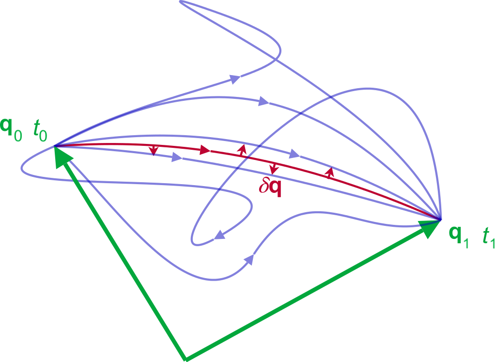
The Euler-Lagrange equation. In order to “deduce the complete mechanics of solid and fluid bodies,” all Lagrange had to do was constrain every path to be a stationary point in \(S\). The modern principle of least action looks very similar: we let \(\mathcal{L} \equiv T - V\) (this is called the Lagrangian), and then write the constraint as \( \frac{d}{dt} \frac{\partial \mathcal{L}}{\partial \dot q_j} = \frac{\partial \mathcal{L}}{\partial q_j}\). Physicists call this constraint equation the Euler-Lagrange equation.
When you first encounter it, the principle of least action can seem abstract and impractical. But it can be quite easy to apply in practice. Consider, for example, a single particle with mass \(m\), position \(q\), and potential energy \(V(q)\):
\(\begin{align} \scriptstyle \mathcal{L} & \scriptstyle ~=~ -V(q) + \frac{1}{2} m \dot q ^2 & \scriptstyle \text{write down the Lagrangian} \quad (2)\\ \scriptstyle -\frac{\partial V(q)}{\partial q} & \scriptstyle ~=~ m \ddot q & \scriptstyle \text{apply Euler-Lagrange} \quad (3)\\ \scriptstyle F & \scriptstyle ~=~ ma & \scriptstyle \text{this is Newton's second law } \quad (4)\\ \end{align}\) \(\begin{align} \mathcal{L} & ~=~ -V(q) + \frac{1}{2} m \dot q ^2 & \text{write down the Lagrangian} \quad (2)\\ -\frac{\partial V(q)}{\partial q} & ~=~ m \ddot q & \text{apply the Euler-Lagrange equation to } \mathcal{L} \quad (3)\\ F & ~=~ ma & \text{this is Newton's second law } \quad (4)\\ \end{align}\)
Nature’s cost function. As a physicist who now does machine learning, I can’t help but think of \(S\) as Nature’s cost function. After all, it is a scalar quantity for which Nature finds a stationary point, usually a minimum, in order to generate the dynamics of the entire universe. The analogy gets even more interesting at small spatial scales, where quantum wavefunctions can be interpreted as Nature’s way of exploring multiple paths that are all very close to the path of stationary action.1
How we usually solve Lagrangians
Ever since Lagrange introduced the notion of stationary action, physicists have followed a simple formula:
- Find analytic expressions for kinetic and potential energy
- Write down the Lagrangian
- Apply the Euler-Lagrange constraint
- Solve the resulting system of differential equations
But these analytic solutions are rather crude approximations of the real world. An alternative approach is to assume that the Lagrangian is an arbitrarily complicated function – a black box that does not permit analytical solutions. When this is the case, we must give up all hope of writing the Lagrangian out by hand. However, there is still a chance that we can parameterize it with a neural network and learn it straight from data. That is the main contribution of our recent paper.
How to learn Lagrangians
The process of learning a Lagrangian differs from the traditional approach, but it also involves four basic steps:
- Obtain data from a physical system
- Parameterize the Lagrangian with a neural network (\(\mathcal{L}\equiv \mathcal{L}_{\theta}\)).
- Apply the Euler-Lagrange constraint
- Backpropagate through the constraint to train a parametric model that approximates the true Lagrangian
The first two steps are fairly straightforward, and we’ll see that automatic differentiation makes the fourth pretty painless. So let’s focus on step 3: applying the Euler-Lagrange constraint. Our angle of attack will be to write down the constraint equation, treat \(\mathcal{L}\) as a differentiable blackbox function, and see whether we can still obtain dynamics:
\(\begin{align} & \scriptstyle \frac{d}{dt} \frac{\partial \mathcal{L}}{\partial \dot q_j} \scriptstyle ~=~ \frac{\partial \mathcal{L}}{\partial q_j} & \scriptstyle \text{Euler-Lagrange } (5)\\ &\scriptstyle \frac{d}{dt} \nabla_{\dot q} \mathcal{L} \scriptstyle ~=~ \nabla_{q} \mathcal{L} & \scriptstyle \text{vectorize } (6)\\ &\scriptstyle \nabla_q \mathcal{L} \scriptstyle ~=~ (\nabla_{\dot q}\nabla_{\dot q}^{\top}\mathcal{L})\ddot q + (\nabla_{q}\nabla_{\dot q}^{\top}\mathcal{L}) \dot q & \scriptstyle \text{expand }\frac{d}{dt} \text{ }(7)\\ &\scriptstyle \ddot q \scriptstyle ~=~ (\nabla_{\dot q}\nabla_{\dot q}^{\top}\mathcal{L})^{-1}[\nabla_q \mathcal{L} - (\nabla_{q}\nabla_{\dot q}^{\top}\mathcal{L})\dot q] & \scriptstyle \text{solve for } \ddot q \text{ }(8)\\ \end{align}\) \(\begin{align} \frac{d}{dt} \frac{\partial \mathcal{L}}{\partial \dot q_j} &= \frac{\partial \mathcal{L}}{\partial q_j} & \text{the Euler-Lagrange equation} \quad (5)\\ \frac{d}{dt} \nabla_{\dot q} \mathcal{L} &= \nabla_{q} \mathcal{L} & \text{switch to vector notation} \quad (6)\\ (\nabla_{\dot q}\nabla_{\dot q}^{\top}\mathcal{L})\ddot q + (\nabla_{q}\nabla_{\dot q}^{\top}\mathcal{L}) \dot q &= \nabla_q \mathcal{L} & \text{expand time derivative }\frac{d}{dt} \quad (7)\\ \ddot q &= (\nabla_{\dot q}\nabla_{\dot q}^{\top}\mathcal{L})^{-1}[\nabla_q \mathcal{L} - (\nabla_{q}\nabla_{\dot q}^{\top}\mathcal{L})\dot q] & \text{matrix inverse to solve for } \ddot q \quad (8)\\ \end{align}\)
For a given set of coordinates \(x_t=(q_t,\dot q_t)\), we now have a method for calculating \(\dot x_t=(\dot q_t,\ddot q_t)\) from a blackbox Lagrangian. We can integrate this quantity to obtain the dynamics of the system. And in the same manner as Hamiltonian Neural Networks, we can learn \(\mathcal{L_{\theta}}\) by differentiating the MSE loss between \(\dot x_t^{\mathcal{L_{\theta}}}\) and \(\dot x_t^{\textrm{true}}\).
Implementation. If you look closely at Equation 8, you may notice that it involves both the Hessian and the gradient of a neural network during the forward pass of the LNN. This is not a trivial operation, but modern automatic differentiation makes things surprisingly smooth. Written in JAX, Equation 8 is just a few lines of code:
q_tt = (
	jax.numpy.linalg.pinv(jax.hessian(lagrangian, 1)(q, q_t)) @ (
		jax.grad(lagrangian, 0)(q, q_t)
		- jax.jacfwd(jax.grad(lagrangian, 1), 0)(q, q_t) @ q_t
	)
)
Learning real Lagrangians
In our paper, we conduct several experiments to validate this approach. In the first, we show that Lagrangian Neural Networks can learn the dynamics of a double pendulum.
Double pendulum. The double pendulum is a dynamics problem that regular neural networks struggle to fit because they have no prior for conserving the total energy of the system. It is also a problem where HNNs struggle, since the canonical coordinates of the system are not trivial to compute (see equations 1 and 2 of this derivation for example). But in contrast to these baseline methods, Figure 4 shows that LNNs are able to learn the Lagrangian of a double pendulum.
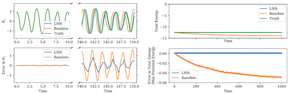
It’s also interesting to compare qualitative results. In the video below, we use a baseline neural network and an LNN to predict the dynamics of a double pendulum, starting from the same initial state. You’ll notice that both trajectories seem reasonable until the end of the video, when the baseline model shifts to states that have much lower total energies.
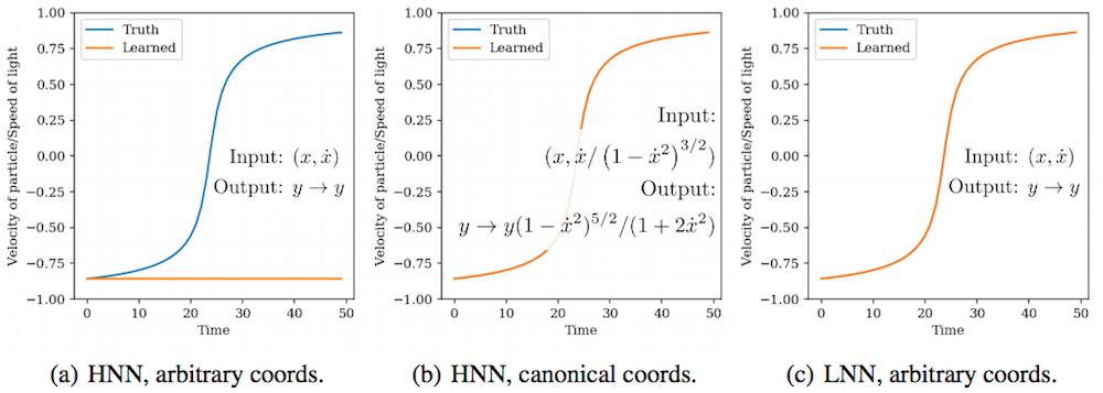
Relativistic particle. Another system we considered was a particle of mass \(m=1\) moving at a relativistic velocity through a potential \(g\) with \(c=1\). The Lagrangian of the system is \(\mathcal{L} = ((1 - \dot{q}^2)^{-1/2} - 1) + g q\) and it is interesting because existing Hamiltonian and Lagrangian learning approaches fail. HNNs fail because the canonical momenta of the system are hard to compute. Deep Lagrangian Networks2 fail because they make restrictive assumptions about the form of the Lagrangian.
Related Work
Learning invariant quantities. This approach is similar in spirit to Hamiltonian Neural Networks (HNNs) and Hamiltonian Generative Networks3 (HGNs). In fact, this blog post was written as a compliment to the original HNN post and it has the same fundamental motivations. Unlike these previous works, our aim here is to learn a Lagrangian rather than a Hamiltonian so as not to restrict the inputs to being canonical coordinates. It’s worth noting that once we learn a Lagrangian, we can always use it to obtain the value of a Hamiltonian using the Legendre transformation.
Deep Lagrangian Networks (DeLaN, ICLR’19). Another closely related work is Deep Lagrangian Networks2 in which the authors show how to learn specific types of Lagrangian systems. They assume that the kinetic energy is an inner product of the velocity, which works well for rigid body dynamics such as those in robotics. However, there are many physical systems that do not have this specific form. Some simple examples include a charged particle in a magnetic field or a fast-moving object with relativistic corrections. We see LNNs as a complement to DeLaNs in that they cover the cases where DeLaNs struggle but are less amenable to robotics applications.
Closing Thoughts
The principle of stationary action is a unifying force in physics. It represents a consistent “law of the universe” which holds true in every system humans have ever studied: from the very small1 to the very large, from the very slow to the very fast. Lagrangian Neural Networks represent a different sort of unification. They aim to strengthen the connection between real-world data and the underlying physical constraints that it obeys. This gives LNNs their own sort of beauty, a beauty that Lagrange himself may have admired.
Footnotes
-
Here \(e^{-S/h}\) is actually the probability of a particular path occurring. Because \(h\) is small, we usually only observe the minimum value of \(S\) on large scales. See Feynman lecture 19 for more on this. ↩ ↩2
-
Lutter, M., Ritter, C., and Peters, J. Deep lagrangian networks: Using physics as model prior for deep learning, International Conference on Learning Representations, 2019. ↩ ↩2
-
Toth, P., Rezende, D. J., Jaegle, A., Racanière, S., Botev, A., & Higgins, I. Hamiltonian Generative Networks, International Conference on Learning Representations, 2020. ↩