Dissipative Hamiltonian Neural Networks

Dissipative HNNs (D-HNNs) improve upon Hamiltonian Neural Networks. They output two scalar functions, denoted here by H and D. The first of these two, H, is the Hamiltonian. We use its symplectic gradient to model energy-conserving dynamics. The second, D, is the Rayleigh dissipation function. We use it to model the dissipative component of the system. The addition of this dissipation function allows D-HNNs to model systems where energy is not quite conserved, as, for example, in the case of the damped mass-spring system shown here.

A sea of change

We are immersed in a complex, dynamic world where change is the only constant. And yet there are certain patterns to this change that suggest natural laws. These laws include conservation of mass, energy, and momentum. Taken together, they constitute a powerful simplifying constraint on reality. Indeed, physics tells us that a small set of laws and their associated invariances are at the heart of all natural phenomena. Whether we are studying weather, ocean currents, earthquakes, or molecular interactions, we should take care to respect these laws. And when we apply learning algorithms to these domains, we should ensure that they, too, respect these laws.

We can do this by building models that are primed to learn invariant quantities from data: these models include HNNs, LNNs, and a growing class of related models. But one problem with these models is that, for the most part, they can only handle data where some quantity (such as energy) is exactly conserved. If the data is collected in the real world and there is even a small amount of friction, then these models struggle. In this post, we introduce Dissipative HNNs, a class of models which can learn conservation laws from data even when energy isn’t perfectly conserved.

We live in a sea of change. But no matter how complex a system's dynamics are, they can always be decomposed into the sum of dissipative dynamics and conservative dynamics.

The core idea is to use a neural network to parameterize both a Hamiltonian and a Rayleigh dissipation function. During training, the Hamiltonian function fits the conservative (rotational) component of the dynamics whereas the Rayleigh function fits the dissipative (irrotational) component. Let’s dive in to how this works.

A quick theory section

The Hamiltonian function. The Hamiltonian \(\mathcal{H}(\textbf{q},\textbf{p})\) is scalar function where by definition \( \frac{\partial \mathcal{H}}{\partial \textbf{p}} = \frac{\partial \textbf{q}}{dt}, -\frac{\partial \mathcal{H}}{\partial \textbf{q}} = \frac{\partial \textbf{p}}{dt} \). This constraint tells us that, even as the position and momentum coordinates of the system \(\textbf{(q, p)}\) change, the scalar output \(\mathcal{H}\) remains fixed. In other words, \(\mathcal{H}\) is invariant with respect to \(\textbf{q}\) and \(\textbf{p}\) as they change over time; it is a conserved quantity. Hamiltonians often appear in physics because for every natural symmetry/law in the universe, there is a corresponding conserved quantity (see Noether’s theorem).

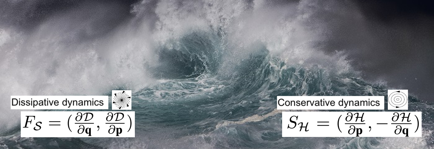
The Rayleigh function. The Rayleigh dissipation function \(\mathcal{D}(\textbf{q},\textbf{p})\) is a scalar function that provides a way to account for dissipative forces such as friction in the context of Hamiltonian mechanics. As an example, the Rayleigh function for linear, velocity-dependent dissipation would be \(\mathcal{D} = \frac{1}{2}\rho\dot{q}^2\) where \(\rho\) is a constant and \(\dot q\) is the velocity coordinate. We add this function to a Hamiltonian whenever the conserved quantity we are trying to model is changing due to sources and sinks. For example, if \(\mathcal{H}\) measures the total energy of a damped mass-spring system, then we could add the \(\mathcal{D}\) we wrote down above to account for the change in total energy due to friction.

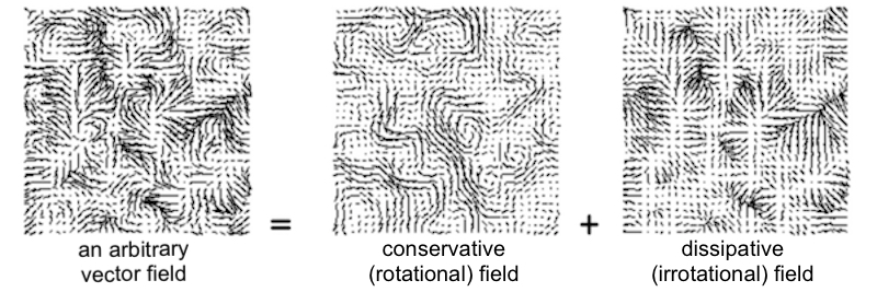
Helmholtz decompositions. Like many students today, Hermann von Helmholtz realized that medicine was not his true calling. Luckily for us, he switched to physics and discovered one of the most useful tools in vector analysis: the Helmholtz decomposition. The Helmholtz decomposition says that any vector field \(V\) can be written as the gradient of a scalar potential \(\phi\) plus the curl of a vector potential \(\mathcal{\textbf{A}}\). In other words, \( V = \nabla\phi + \nabla\times \mathcal{\textbf{A}}\). Note that the first term is irrotational and the second term is rotational. This tells us that any vector field can be decomposed into the sum of an irrotational (dissipative) vector field and a rotational (conservative) vector field. Here’s a visual example:

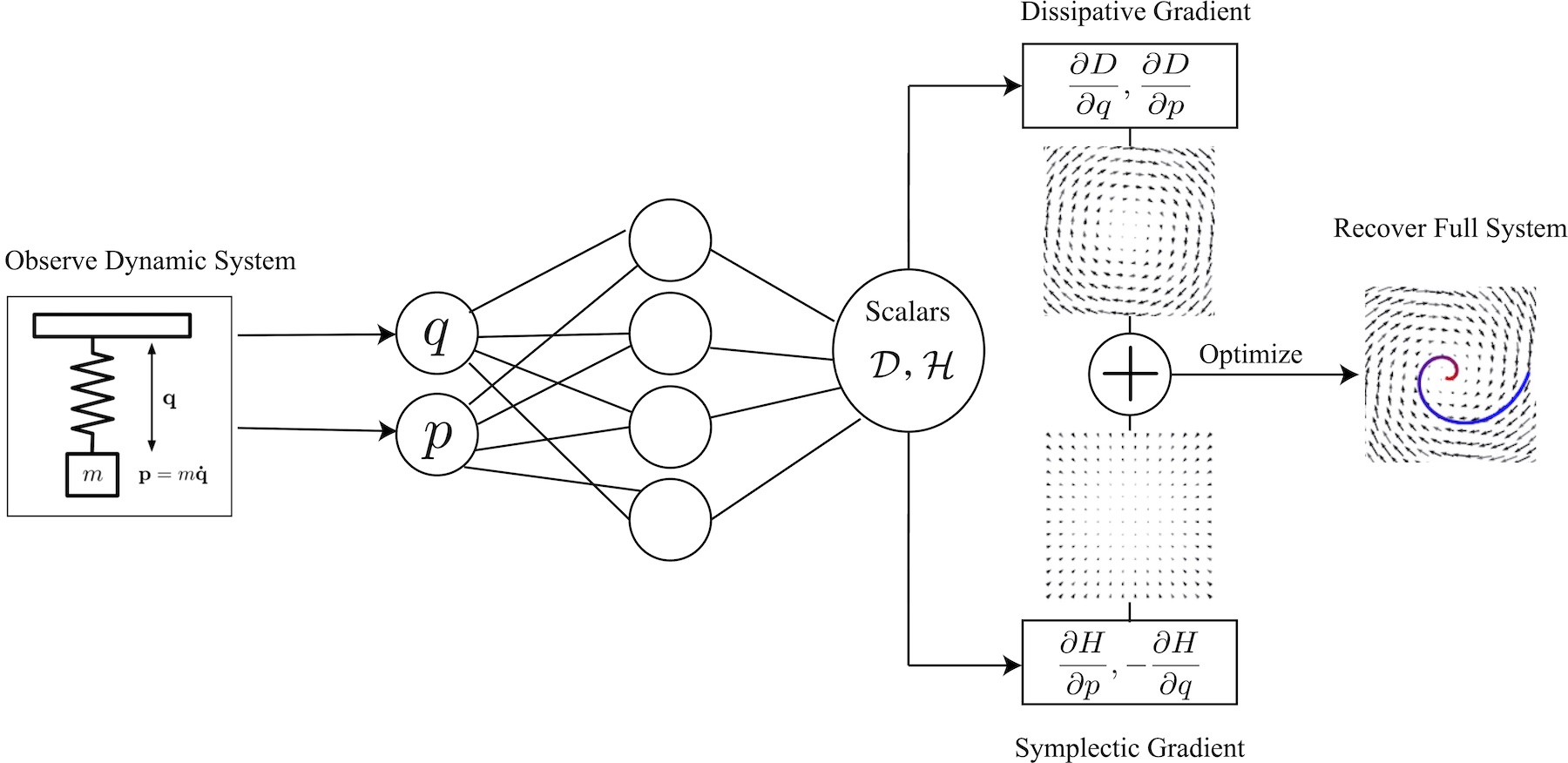
Putting it together. In Hamiltonian Neural Networks, we showed how to parameterize the Hamiltonian function and then learn it directly from data. Here, we parameterize a Rayleigh function as well. Our model looks the same as an HNN except now it has a second scalar output which we use for the Rayleigh function (see the first image in this post). During the forward pass, we take the symplectic gradient of the Hamiltonian to obtain conservative forces. Note that as we do this, the symplectic gradient constitutes a rotational vector field over the model’s inputs. During the forward pass we also take the gradient of the Rayleigh function to obtain dissipative forces. This gradient gives us an irrotational vector field over the same domain.

All of this means that, by construction, our model will learn an implicit Helmholtz decomposition of the forces acting on the system.

An introductory model

We coded up a D-HNN model and used it to fit three physical systems: a synthetic damped mass-spring, a real-world pendulum, and an ocean current timeseries sampled from the OSCAR dataset. In this post, we’ll focus on the damped mass-spring example in order to build intuition for how D-HNNs work.

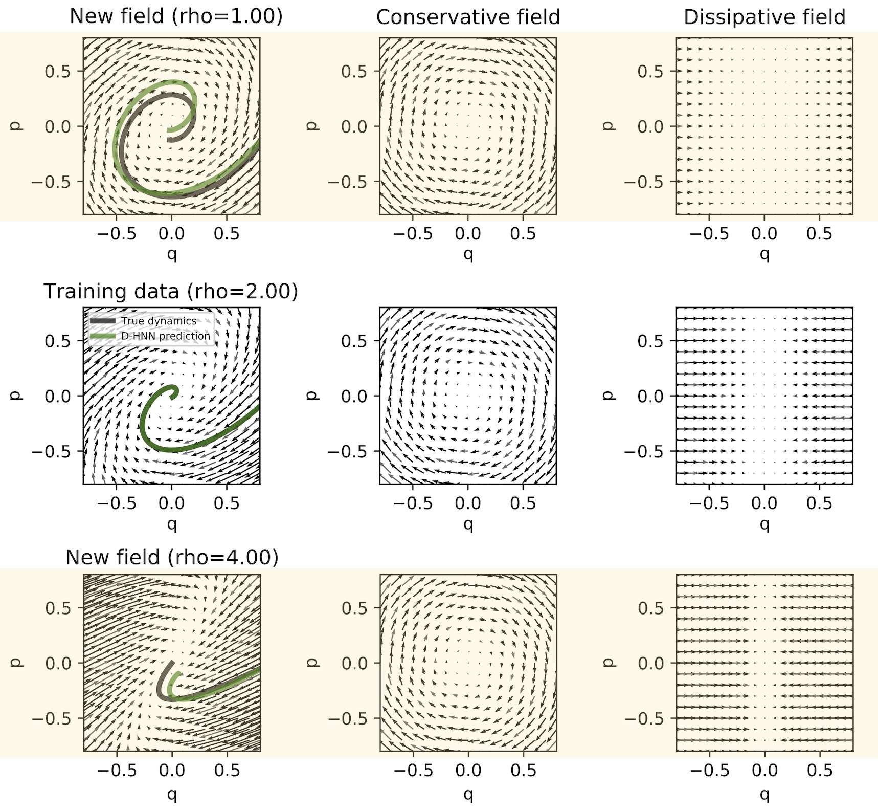
We can describe the state of a damped (one dimensional) mass-spring system with just two coordinates, \(q\) and \(p\). Also, we can plot these coordinates on Cartesian \(x\) and \(y\) axes to obtain phase-space diagrams. These diagrams are useful because they allow us to visualize and compare our model to other baseline models.

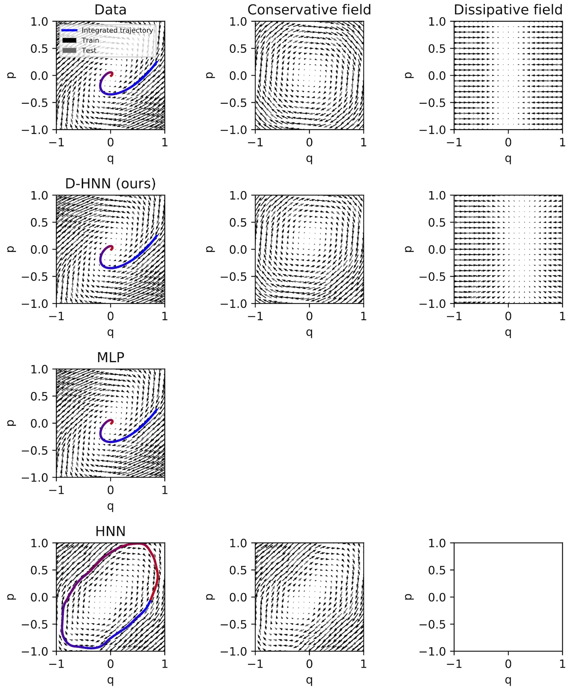
In the image above, the damped mass-spring dataset is plotted in the upper left square. Each arrow represents the time derivative of the system with respect to that \((p,q)\) coordinate. The Helmholtz decomposition tells us that this vector field can be decomposed into conservative and dissipative components, and indeed that is what we have done in the second and third columns.¹ You may notice that the dissipative field in the third column isolates the force due to friction.

In the second row, we evaluate a D-HNN trained on the system. The D-HNN produces a trajectory that closely matches ground truth. By plotting the symplectic gradient of \(\mathcal{H}\) and the gradient of \(\mathcal{D}\), we can see that it has properly decoupled the conservative and dissipative dynamics respectively. By contrast, in the third row, we train a baseline model (an MLP) on the same data; this model produces a good trajectory but is unable to learn conservative and dissipative dynamics separately. Finally, in the fourth row, we train an HNN on the same dataset and find that it is only able to model the conservative component of the system’s dynamics. It strictly enforces conservation of energy in a scenario where energy is not actually conserved, leading to a poor prediction.

Why decouple conservative and dissipative dynamics?

We’ve described a model that can learn conservative and dissipative dynamics separately and shown that it works on a toy problem. Why is this a good idea? One answer is that it lets our model fit data in a more physically-realistic manner, leading to better generalization.

If we were to suddenly double the coefficient of friction \(\rho\), our MLP model would not be able to predict a viable trajectory. This is because it models the dissipative and conservative dynamics of the system together. However, since our D-HNN learned these dynamics separately, it can generalize to new friction coefficients without additional training. In order to double the scale of dissipative forces, we can simply multiply the gradient of the Rayleigh function by two. The image below shows how this produces viable trajectories under unseen friction coefficients (orange highlights).

Additional experiments

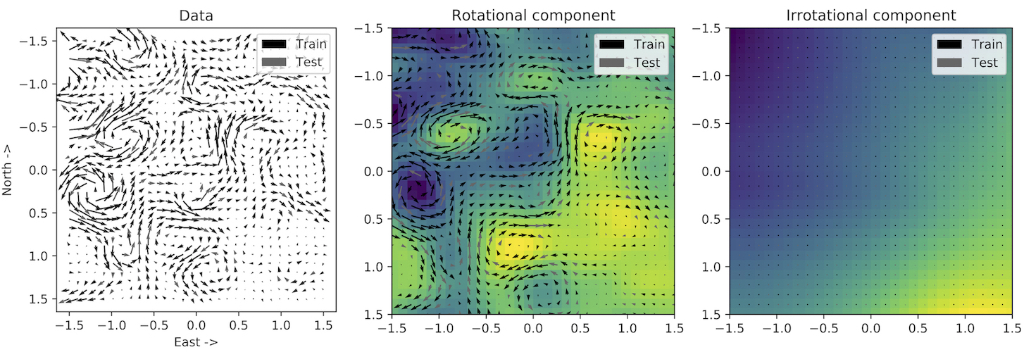
We also trained our model on data from a real pendulum and ocean current data from the OSCAR dataset (shown below). On these larger and more more difficult tasks, our model continued to decouple conservative and dissipative dynamics. The details and results are outside the scope of this post, but you can find them in our paper.

Closing thoughts

This work is a small, practical contribution to science in that it proposes a new physics prior for machine learning models. But it is also a step towards a larger and more ambitious goal: that of building models which can extract conservation laws directly from noisy real-world data. We hope that future work in this direction will benefit from our findings.

Footnotes