Six Experiments in Action Minimization
In a recent post, we used gradient descent to find the path of least action for a free body. That this worked at all was interesting – but some important questions remain. For example: how well does this approach transfer to larger, more nonlinear, and more chaotic systems? That is the question we will tackle in this post.
Six systems
In order to determine how action minimization works on more complex systems, we studied six systems of increasing complexity. The first of these was the free body, which served as a minimal working example, useful for debugging. The next system was a simple pendulum – another minimal working example, but this time with periodic nonlinearities and radial coordinates.
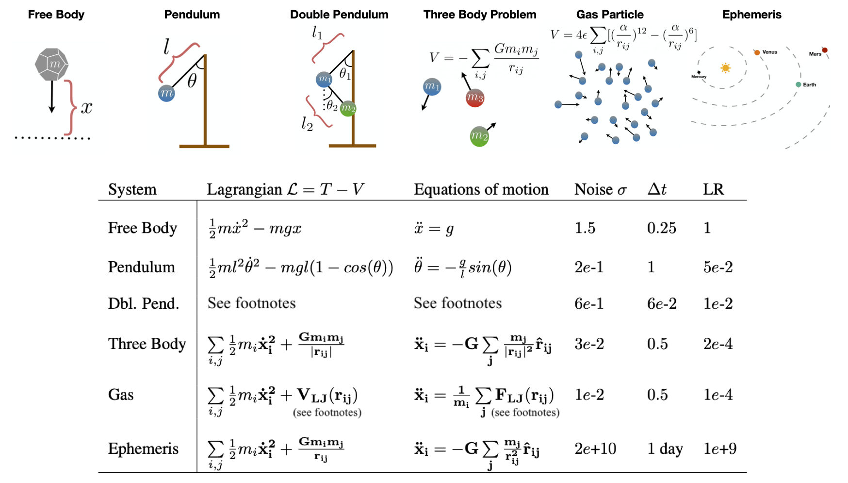
Once we had tuned our approach on these two simple systems, we turned our attention to four more complex systems: a double pendulum, the three body problem, a simple gas, and a real ephemeris dataset of planetary motion (the orbits were projected onto a 2D plane). These systems presented an interesting challenge because they were all nonlinear, chaotic, and high-dimensional.1 In each case, we compared our results to a baseline path obtained with a simple ODE solver using Euler integration.
The unconstrained energy effect
Early in our experiments we encountered the unconstrained energy effect. This happens when the optimizer converges on a valid physical path with a different total energy from the baseline. The figure below shows an example. The reason this happens is that, although we fix the initial and final states, we do not constrain the path’s total energy \(T+V\). Even though paths like the one shown below are not necessarily invalid, they make it difficult for us to recover baseline paths.
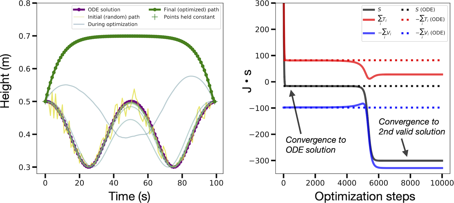
For this reason, we used the baseline ODE paths to initialize our paths, perturbed them with Gaussian noise, and then used early stopping to select for paths which were similar (often, identical) to the ODE baselines. This approach matched the mathematical ansatz of the “calculus of variations” where one studies perturbed paths in the vicinity of the true path. We note that there are other ways to mitigate this effect which don’t require an ODE-generated initial path.2
Results
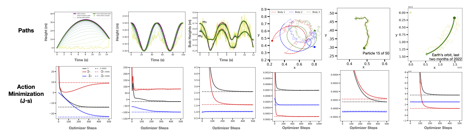
On all six physical systems we obtained paths of least action which were nearly identical to the baseline paths. In the figure below you can also see the optimization dynamics. Our results suggest that action minimization can generate physically-valid dynamics even for chaotic and strongly-coupled systems like the double pendulum and three body problem. One interesting pattern we noticed was that optimization dynamics were dominated by the kinetic energy term \(T\). This occured because \(S\) tended to be more sensitive to \(T\) (which grew as \({\bf \dot{x}}^2\)) than \(V\).
Applications
The goal of this post was just to demonstrate that action minimization scales to larger problems. Nevertheless, we can’t help but take a moment to speculate on potential applications of this method:
- ODE super-resolution. If one were to obtain a low-resolution trajectory via a traditional integration method such as Euler integration, one could then upsample the path by a factor of 10 to 100 (using, eg, linear interpolation) and then run action minimization to make it physically-valid. This procedure would take less time than using the ODE integrator alone.
- Infilling missing data. Many real-world datasets have periods of missing data. These might occur due to a sensor malfunction, or they might be built into the experimental setup – for example, a satellite can’t image clouds and weather patterns as well at night – either way, action minimization is well-suited for inferring the sequence of states that connect a fixed start and end state. Doing this with an ODE integrator, meanwhile, is not as natural because there’s no easy way to incorporate the known end state into the problem definition.
- When the final state is irrelevant. There are many simulation scenarios where the final state is not important at all. What really matters is that the dynamics look realistic in between times \(t_1\) and \(t_2\). This is the case for simulated smoke in a video game: the smoke just needs to look realistic. With that in mind, we could choose a random final state and then minimize the action of the intervening states. This could allow us to obtain realistic graphics more quickly than numerical methods that don’t fix the final state.
Discussion
Action minimization shows how the action really does act like a cost function. This isn’t something you’ll hear in your physics courses, even most high-level ones. And yet, it’s an elegant and accurate way to view physics. In a future post, we’ll see how this notion extends even into quantum mechanics.
Footnotes
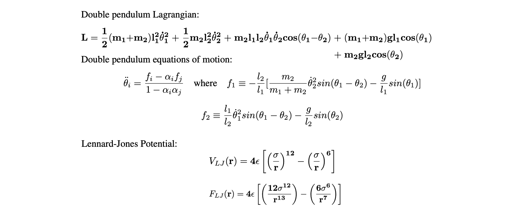
The double pendulum and Lennard-Jones potentials were too long to fit into the table above. Here they are: